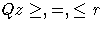
Linear Programming Models: Interior Point Algorithm
By default, the Interior Point algorithm is used for problems without a network
component, that is, a Linear Programming problem.
You do not need to specify the
INTPOINT option in the
PROC NETFLOW statement (although you will do no harm if you do).
Data for a linear programming problem resembles the data for side constraints
and nonarc variables supplied to PROC NETFLOW when solving a constrained network problem.
It is also very similar to the data required by the LP procedure.
If the network component of NPSC is removed,
the result is the mathematical description of the
Linear Programming problem.
If an LP has
g variables, and
k constraints, then
the formal statement of the problem solved by PROC NETFLOW is
-
- min {dT z}
- subject to
-

-
- where
-
d
is the g x 1 objective function coefficient of
variables vector.
-
z
is the g x 1 variable value vector.
-
Q
is the k x g constraint coefficient matrix for
variables, where
Qi,j is the coefficient of variable j in the ith
constraint.
-
r
is the k x 1 side constraint right-hand-side vector.
-
m is the g x 1 variable value lower bound
vector.
-
v is the g x 1 variable
value upper bound vector.
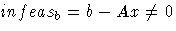
After preprocessing, the Linear Program to be solved is
-
- min {cT x}
- subject to
- A x = b
-

This is the
primal problem.
The matrices of d z Q of NP have been renamed
c x and A respectively, as these symbols are by convention
used more, the problem to be solved is different from the original because of
preprocessing,
and there has been a change of primal variable to transform the
LP into one whose variables have zero lower bounds.
To simplify the algebra here, assume that variables have infinite bounds,
and constraints are equalities.
(Interior Point algorithms do efficiently handle finite bounds, and
it is easy to introduce primal slack variables to change inequalities into
equalities.) The problem has n variables. i is a variable number.
k is an iteration number, and if used as a subscript or superscript
denotes "of iteration k".
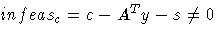
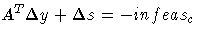
There exists an equivalent problem, the dual problem, stated as
-
- max {bT y}
- subject to
- AT y + s = c
-

- where
- y are dual variables, and s are dual constraint slacks
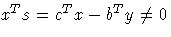
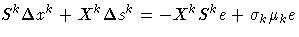
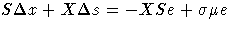
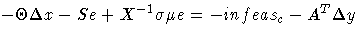
What the Interior Point has to do is solve the system of equations to
satisfy the Karush-Kuhn-Tucker (KKT) conditions for optimality:
-
- A x = b
-
- AT y + s = c
-
- xT s = 0
-
-
These are the conditions for feasibility, with the complementarity
condition xT s = 0 added. cT x = bT y must occur at the optimum.
Complementarity forces the optimal objectives of the primal and dual
to be equal, cT xopt = bT yopt, as
-
- 0 = xTopt sopt = sTopt xopt = (c - AT yopt)T xopt = cT xopt -
yTopt (A xopt) = cT xopt - bT yopt
-
- 0 = cT xopt - bT yopt
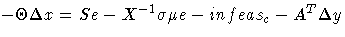
Before the optimum is reached, a solution (x, y, s) may not satisfy the KKT conditions.
- Primal constraints can be broken,
 .
.
- Dual constraints can be broken,
 .
.
- Complementarity is unsatisfied,
 .This is called the duality gap.
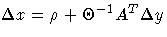
Interior Point algorithm works by using Newtons method to find a
direction
to move 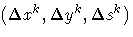 from the current solution (xk, yk, sk) toward a better solution.
-

 is the step length and is assigned a value as large as possible but
  and not so
large that a xk+1i or sk+1i
is "too close" to zero.
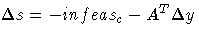
The direction in which to move is found using
and not so
large that a xk+1i or sk+1i
is "too close" to zero.
The direction in which to move is found using
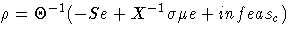
-
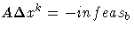
-
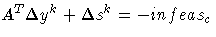
-
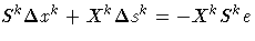
- where
- S = diag(s), X = diag(x), and e = vector with all elements = 1
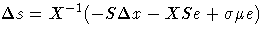
To greatly improve performance, the third equation is changed to
-
- where
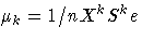 , the average complementarity, and
-

The effect now is to find a direction in which to move to reduce
infeasibilities and to reduce the complementarity toward zero,
but if any
xki ski is too close to zero, it is "nudged out" to  ,any
xki ski that is larger than is "nudged into" .A
,any
xki ski that is larger than is "nudged into" .A  close to or equal to 0.0 biases a direction toward the
optimum,
and a value for close to or equal to 1.0 "centers" the
direction toward a point where all pairwise products
close to or equal to 0.0 biases a direction toward the
optimum,
and a value for close to or equal to 1.0 "centers" the
direction toward a point where all pairwise products  .Such points make up the Central Path in the interior.
Although centering directions make little, if any, progress in reducing
and moving the solution closer to the optimum,
substantial progress toward the optimum can usually be made in
the next iteration.
.Such points make up the Central Path in the interior.
Although centering directions make little, if any, progress in reducing
and moving the solution closer to the optimum,
substantial progress toward the optimum can usually be made in
the next iteration.
The Central Path is crucial to why the Interior Point algorithm is so
efficient. This path "guides"
the algorithm to the optimum through the interior of feasible space.
Without centering, the algorithm would find a series of solutions near each other
close to the boundary of feasible space.
Step lengths along the direction
would be small and many
more iterations would probably be required to reach the optimum.
That in a nutshell is the Primal-Dual Interior Point algorithm.
Varieties of the algorithm differ in the way and are chosen
and the direction adjusted each iteration.
A wealth of information can be found in the texts by Roos, Terlaky, and Vial 1997,
Wright 1996, and Ye 1996.
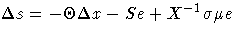
The calculation of the direction is the most time-consuming step
of the Interior Point algorithm.
Assume the kth iteration is being performed,
so the subscript and superscript k can be dropped from the algebra.
-
-
-
Rearranging the second equation
-
Rearranging the third equation
-
-
- where

Equating these two expressions for  and rearranging
-
-
-

-
- where
Substituting into the first direction equation
-
-
-
-
 ,
,  ,
,  ,
,  and are calculated
in that order.
The hardest term is the factorization of the
and are calculated
in that order.
The hardest term is the factorization of the
 matrix
to determine .
Fortunately, although the values of is
different each iteration,
the locations of the nonzeroes in this matrix remain fixed; the
nonzero locations is the same as those in the matrix (A AT).
This is due to
matrix
to determine .
Fortunately, although the values of is
different each iteration,
the locations of the nonzeroes in this matrix remain fixed; the
nonzero locations is the same as those in the matrix (A AT).
This is due to  being a diagonal
matrix that has the effect of merely scaling the columns of (A AT).
being a diagonal
matrix that has the effect of merely scaling the columns of (A AT).
The fact that the nonzeroes in  has a constant pattern is exploited by all
Interior Point algorithms, and is a major reason for their
excellent performance.
Before iterations begin, A AT is examined and it's rows and
columns permutated so that during Cholesky Factorization, the number of
fillins created is smaller.
A list of arithmetic operations to perform the factorization is saved
in concise computer data structures (working with
memory locations rather than actual numerical values).
This is called symbolic factorization.
During iterations, when memory has been initialized with numerical values,
the operations list is performed sequentially.
Determining how the factorization should be performed again and again
is unnecessary.
has a constant pattern is exploited by all
Interior Point algorithms, and is a major reason for their
excellent performance.
Before iterations begin, A AT is examined and it's rows and
columns permutated so that during Cholesky Factorization, the number of
fillins created is smaller.
A list of arithmetic operations to perform the factorization is saved
in concise computer data structures (working with
memory locations rather than actual numerical values).
This is called symbolic factorization.
During iterations, when memory has been initialized with numerical values,
the operations list is performed sequentially.
Determining how the factorization should be performed again and again
is unnecessary.
To solve linear programming problem using
PROC NETFLOW, you save a representation of the variables
and the constraints in one or two SAS data sets. These
data sets are then passed to PROC NETFLOW for solution.
There are various forms that a problem's data can take.
You can use any one or a combination of several of these forms.
The ARCDATA= data set contains information about the variables
of the problem.
Although this data set is called ARCDATA, it contains data for no arcs.
Instead, all data in this data set are related
to variables.
The ARCDATA= data set can be used to specify information about
variables, including objective function coefficients,
lower and upper value bounds, and names.
These data are the elements of the vectors
d, m, and v in problem (NP).
Data for an variable can be given in more than
one observation.
When the data for a constrained network problem is being provided,
the ARCDATA= data set always contains
information necessary for arcs, their tail and head nodes, and optionally
the supply and demand information of these nodes.
When the data for a linear programming problem is being provided,
none of this information is present, as the model has no arcs.
This is the way PROC NETFLOW decides which type of problem it is to solve.
PROC NETFLOW was originally designed to solve models with networks, so an
ARCDATA= data set is always expected.
If an ARCDATA= data set
is not specified, by default the last data set created before
PROC NETFLOW is envoked is assumed to be an
ARCDATA= data set.
However, these characteristics of PROC NETFLOW are not helpful when a
Linear Programming problem is being solved and all data is provided in a
single data set specified by the
CONDATA= data set,
and that data set is not the last data set created before PROC NETFLOW starts.
In this case, you must specify that an
ARCDATA= data set and
a CONDATA= data set are both equal to
the input data set.
PROC NETFLOW then knows that a Linear Programming problem is to be solved,
and the data reside in one data set.
The CONDATA= data set describes
the constraints and
their right-hand-sides. These data are elements of the matrix
Q and
the vector r.
Constraint types are also specified in the CONDATA= data set.
You can include in this data set variable data such as upper bound values,
lower value bounds, and objective function
coefficients. It is possible to give all information about
some or all variables in the CONDATA= data set.
A variable is identified in this data set by its name.
If you
specify a variable's name in the ARCDATA= data set, then this
name is used to associate data in the
CONDATA= data set with
that variable.
If you use the dense constraint input format,
these variable names are names of SAS variables in the
VAR list of the
CONDATA= data set.
If you use the sparse constraint input format,
these variable names are values of the COLUMN
list SAS variable of
CONDATA= data set.
When using the Interior Point algorithm, the execution of PROC NETFLOW
has two stages.
In the preliminary
(zeroth) stage, the data
are read from the
ARCDATA= data set (if used) and the CONDATA= data set.
Error checking is performed.
In the next stage, the Linear Program is preprocessed, then the optimal optimal solution to
the Linear Program is found.
The solution is saved in the
CONOUT= data set.
This data set is also named in the
PROC NETFLOW,
RESET, and
SAVE statements.
See the "Getting Started: Network Models: Interior Point algorithm" section for a fuller description
of the stages of the Interior Point algorithm.
Introductory Example:
Linear Programming Models: Interior Point algorithm
Consider the Linear Programming problem in the "An Introductory Example" section
in the chapter on the LP procedure.
data dcon1;
   input _id_ $14.
         a_light a_heavy brega naphthal naphthai
         heatingo jet_1 jet_2
         _type_ $ _rhs_;
   datalines;
profit         -175 -165 -205  0  0  0 300 300 max     .
naphtha_l_conv .035 .030 .045 -1  0  0   0   0  eq     0
naphtha_i_conv .100 .075 .135  0 -1  0   0   0  eq     0
heating_o_conv .390 .300 .430  0  0 -1   0   0  eq     0
recipe_1          0    0    0  0 .3 .7  -1   0  eq     0
recipe_2          0    0    0 .2  0 .8   0  -1  eq     0
available       110  165   80  .  .  .   .   . upperbd .
;
To find the minimum cost solution
and to examine all or parts of the optimum, you use
PRINT statements.
- print problem/short; outputs information for all
variables and all constraint coefficients. See Figure 4.19.
- print some_variables(j:)/short; is information about a set of variables,
(in this case, those with names that start with the character string (here, the single character "j" (without the quotes))
preceeding the colon.
See Figure 4.20.
- print some_cons(recipe_1)/short; is information about a set of constraints
(here, that set only has one member, the constraint called recipe_1).
See Figure 4.21.
- print con_variables(_all_,brega)/short; lists the constraint information for a set of variables
(here, that set only has one member, the variable called brega).
See Figure 4.22.
- print con_variables(recipe:,n: jet_1)/short; coefficient information
for those in a set of constraints belonging to a set of variables.
See Figure 4.23.
   proc netflow
      condata=dcon1
      conout=solutn1;
   run;
print problem/short;
print some_variables(j:)/short;
print some_cons(recipe_1)/short;
print con_variables(_all_,brega)/short;
print con_variables(recipe:,n: jet_1)/short;
The following messages, that appear on the SAS log, summarize
the model as read by PROC NETFLOW and note the progress toward a
solution:
NOTE: Number of variables= 8 .
NOTE: Number of <= constraints= 0 .
NOTE: Number of == constraints= 5 .
NOTE: Number of >= constraints= 0 .
NOTE: Number of constraint coefficients= 18 .
NOTE: 0 columns, 0 rows and 0 coefficients were added
      to the problem to handle unrestricted variables,
      variables that are split, and constraint slack or
      surplus variables.
NOTE: There are 8 nonzero elements in A * A transpose.
NOTE: Number of fill-ins=0.
NOTE: Of the 5 rows and columns, 0 are sparse.
NOTE: There are 0 nonzero elements in the sparse rows of
      the factored A * A transpose. This includes fill-ins
      in the sparse rows.
NOTE: There are 0 operations of the form
      u[i,j]=u[i,j]-u[q,j]*u[q,i]/u[q,q] to factorize the
      sparse rows of A * A transpose.
NOTE: Constraint feasibility attained by iteration 3.
NOTE: Bound feasibility attained by iteration 3.
NOTE: Dual feasibility attained by iteration 3.
NOTE: Primal-Dual Predictor-Corrector Interior point
      algorithm performed 8 iterations.
NOTE: Objective = 1544.0000121.
NOTE: The data set WORK.SOLUTN1 has 8 observations and
      6 variables.
|
| _N_ |
_NAME_ |
_OBJFN_ |
_UPPERBD |
_LOWERBD |
_VALUE_ |
| 1 |
a_heavy |
-165 |
165 |
0 |
5.583E-7 |
| 2 |
a_light |
-175 |
110 |
0 |
110 |
| 3 |
brega |
-205 |
80 |
0 |
80 |
| 4 |
heatingo |
0 |
99999999 |
0 |
77.3 |
| 5 |
jet_1 |
300 |
99999999 |
0 |
60.65 |
| 6 |
jet_2 |
300 |
99999999 |
0 |
63.33 |
| 7 |
naphthai |
0 |
99999999 |
0 |
21.8 |
| 8 |
naphthal |
0 |
99999999 |
0 |
7.45 |
|
|
| _N_ |
_id_ |
_type_ |
_rhs_ |
_NAME_ |
_COST_ |
_CAPAC_ |
_LO_ |
_VALUE_ |
_COEF_ |
| 1 |
heating_o_conv |
EQ |
0 |
a_heavy |
-165 |
165 |
0 |
5.583E-7 |
0.3 |
| 2 |
heating_o_conv |
EQ |
0 |
a_light |
-175 |
110 |
0 |
110 |
0.39 |
| 3 |
heating_o_conv |
EQ |
0 |
brega |
-205 |
80 |
0 |
80 |
0.43 |
| 4 |
heating_o_conv |
EQ |
0 |
heatingo |
0 |
99999999 |
0 |
77.3 |
-1 |
| 5 |
naphtha_i_conv |
EQ |
0 |
a_heavy |
-165 |
165 |
0 |
5.583E-7 |
0.075 |
| 6 |
naphtha_i_conv |
EQ |
0 |
a_light |
-175 |
110 |
0 |
110 |
0.1 |
| 7 |
naphtha_i_conv |
EQ |
0 |
brega |
-205 |
80 |
0 |
80 |
0.135 |
| 8 |
naphtha_i_conv |
EQ |
0 |
naphthai |
0 |
99999999 |
0 |
21.8 |
-1 |
| 9 |
naphtha_l_conv |
EQ |
0 |
a_heavy |
-165 |
165 |
0 |
5.583E-7 |
0.03 |
| 10 |
naphtha_l_conv |
EQ |
0 |
a_light |
-175 |
110 |
0 |
110 |
0.035 |
| 11 |
naphtha_l_conv |
EQ |
0 |
brega |
-205 |
80 |
0 |
80 |
0.045 |
| 12 |
naphtha_l_conv |
EQ |
0 |
naphthal |
0 |
99999999 |
0 |
7.45 |
-1 |
| 13 |
recipe_1 |
EQ |
0 |
heatingo |
0 |
99999999 |
0 |
77.3 |
0.7 |
| 14 |
recipe_1 |
EQ |
0 |
jet_1 |
300 |
99999999 |
0 |
60.65 |
-1 |
| 15 |
recipe_1 |
EQ |
0 |
naphthai |
0 |
99999999 |
0 |
21.8 |
0.3 |
| 16 |
recipe_2 |
EQ |
0 |
heatingo |
0 |
99999999 |
0 |
77.3 |
0.8 |
| 17 |
recipe_2 |
EQ |
0 |
jet_2 |
300 |
99999999 |
0 |
63.33 |
-1 |
| 18 |
recipe_2 |
EQ |
0 |
naphthal |
0 |
99999999 |
0 |
7.45 |
0.2 |
|
Figure 4.19: print problem/short;
|
| _N_ |
_NAME_ |
_COST_ |
_CAPAC_ |
_LO_ |
_VALUE_ |
| 1 |
jet_1 |
300 |
99999999 |
0 |
60.65 |
| 2 |
jet_2 |
300 |
99999999 |
0 |
63.33 |
|
Figure 4.20: print some_variables(j:)/short;
|
| _N_ |
_id_ |
_type_ |
_rhs_ |
_NAME_ |
_COST_ |
_CAPAC_ |
_LO_ |
_VALUE_ |
_COEF_ |
| 1 |
recipe_1 |
EQ |
0 |
heatingo |
0 |
99999999 |
0 |
77.3 |
0.7 |
| 2 |
recipe_1 |
EQ |
0 |
jet_1 |
300 |
99999999 |
0 |
60.65 |
-1 |
| 3 |
recipe_1 |
EQ |
0 |
naphthai |
0 |
99999999 |
0 |
21.8 |
0.3 |
|
Figure 4.21: print some_cons(recipe_1)/short;
|
| _N_ |
_id_ |
_type_ |
_rhs_ |
_NAME_ |
_COST_ |
_CAPAC_ |
_LO_ |
_VALUE_ |
_COEF_ |
| 1 |
heating_o_conv |
EQ |
0 |
brega |
-205 |
80 |
0 |
80 |
0.43 |
| 2 |
naphtha_i_conv |
EQ |
0 |
brega |
-205 |
80 |
0 |
80 |
0.135 |
| 3 |
naphtha_l_conv |
EQ |
0 |
brega |
-205 |
80 |
0 |
80 |
0.045 |
|
Figure 4.22: print con_variables(_all_,brega)/short;
|
| _N_ |
_id_ |
_type_ |
_rhs_ |
_NAME_ |
_COST_ |
_CAPAC_ |
_LO_ |
_VALUE_ |
_COEF_ |
| 1 |
recipe_1 |
EQ |
0 |
jet_1 |
300 |
99999999 |
0 |
60.65 |
-1 |
| 2 |
recipe_1 |
EQ |
0 |
naphthai |
0 |
99999999 |
0 |
21.8 |
0.3 |
| 3 |
recipe_2 |
EQ |
0 |
naphthal |
0 |
99999999 |
0 |
7.45 |
0.2 |
|
Figure 4.23: print con_variables(recipe:,n: jet_1)/short;
Unlike PROC LP, that displays the solution and other information as output,
PROC NETFLOW saves the optimum in output SAS data sets you specify.
For this example, the solution is saved in the SOLUTION data set. It can be
displayed with PROC PRINT as
   proc print data=solutn1;
      var _name_ _cost_ _capac_ _lo_ _flow_ _fcost_;
      sum _fcost_;
      title3 'LP Optimum'; run;
Notice, in the CONOUT=SOLUTION (Figure 4.24), the optimal value
through each variable in the Linear program
is given in the variable named _FLOW_, and the cost of value
for each variable is given in the variable _FCOST_.
|
| Obs |
_NAME_ |
_COST_ |
_CAPAC_ |
_LO_ |
_FLOW_ |
_FCOST_ |
| 1 |
a_heavy |
-165 |
165 |
0 |
0.000 |
-0.00 |
| 2 |
a_light |
-175 |
110 |
0 |
110.000 |
-19250.00 |
| 3 |
brega |
-205 |
80 |
0 |
80.000 |
-16400.00 |
| 4 |
heatingo |
0 |
99999999 |
0 |
77.300 |
0.00 |
| 5 |
jet_1 |
300 |
99999999 |
0 |
60.650 |
18195.00 |
| 6 |
jet_2 |
300 |
99999999 |
0 |
63.330 |
18999.00 |
| 7 |
naphthai |
0 |
99999999 |
0 |
21.800 |
0.00 |
| 8 |
naphthal |
0 |
99999999 |
0 |
7.450 |
0.00 |
| |
|
|
|
|
|
1544.00 |
|
Figure 4.24: CONOUT=SOLUTN1
The same model can be specified in the sparse format as in the
following scon2 dataset.
This format enables you to omit the zero coefficients.
data scon2;
   input _type_ $ @10 _col_ $13. @24 _row_ $16. _coef_;
   datalines;
max      .             profit                    .
eq       .             napha_l_conv              .
eq       .             napha_i_conv              .
eq       .             heating_oil_conv          .
eq       .             recipe_1                  .
eq       .             recipe_2                  .
upperbd  .             available                 .
.        a_light       profit                 -175
.        a_light       napha_l_conv           .035
.        a_light       napha_i_conv           .100
.        a_light       heating_oil_conv       .390
.        a_light       available               110
.        a_heavy       profit                 -165
.        a_heavy       napha_l_conv           .030
.        a_heavy       napha_i_conv           .075
.        a_heavy       heating_oil_conv       .300
.        a_heavy       available               165
.        brega         profit                 -205
.        brega         napha_l_conv           .045
.        brega         napha_i_conv           .135
.        brega         heating_oil_conv       .430
.        brega         available                80
.        naphthal      napha_l_conv             -1
.        naphthal      recipe_2                 .2
.        naphthai      napha_i_conv             -1
.        naphthai      recipe_1                 .3
.        heatingo      heating_oil_conv         -1
.        heatingo      recipe_1                 .7
.        heatingo      recipe_2                 .8
.        jet_1         profit                  300
.        jet_1         recipe_1                 -1
.        jet_2         profit                  300
.        jet_2         recipe_2                 -1
;
To find the minimum cost solution, invoke PROC NETFLOW
(note the SPARSECONDATA option which must be specified) as follows:
   proc netflow
      sparsecondata
      condata=scon2
      conout=solutn2;
   run;
A data set that is used as an
ARCDATA= data set
can be initialized as follows:
data vars3;
   input _name_ $ profit available;
   datalines;
a_heavy  -165 165
a_light  -175 110
brega    -205  80
heatingo    0   .
jet_1     300   .
jet_2     300   .
naphthai    0   .
naphthal    0   .
;
The following CONDATA= data set is the original
dense format CONDATA= dcon1 data set
with the variable information removed.
(You could have left some or all of that information in
CONDATA as PROC NETFLOW "merges" data, but doing that and checking for
consistency uses time.)
data dcon3;
   input _id_ $14.
         a_light a_heavy brega naphthal naphthai
         heatingo jet_1 jet_2
         _type_ $ _rhs_;
   datalines;
naphtha_l_conv .035 .030 .045 -1  0  0   0   0  eq     0
naphtha_i_conv .100 .075 .135  0 -1  0   0   0  eq     0
heating_o_conv .390 .300 .430  0  0 -1   0   0  eq     0
recipe_1          0    0    0  0 .3 .7  -1   0  eq     0
recipe_2          0    0    0 .2  0 .8   0  -1  eq     0
;
It is important to note that it is now necessary to specify the
MAXIMIZE option; otherwise, PROC NETFLOW will
optimize to the minimum
(which, incidently, has a total objective = -3539.25).
You must indicate that the SAS variable profit in the
ARCDATA= vars3 data set has values that are
objective function coefficients, by specifying the
OBJFN statement.
The UPPERBD must be specified as the SAS
variable available that has as values upper bounds.
proc netflow
   maximize             /* ***** necessary ***** */
   arcdata=vars3
   condata=dcon3
   conout=solutn3;
objfn profit;
upperbd available;
run;
The ARCDATA=vars3 data set can become more concise by noting that the model variables
heatingo, naphthai, and naphthal have zero objective function coefficients
(the default) and
default upper bounds, so those observations need not be present.
data vars4;
   input _name_ $ profit available;
   datalines;
a_heavy  -165 165
a_light  -175 110
brega    -205  80
jet_1     300   .
jet_2     300   .
;
The CONDATA=dcon3 data set can become more
concise by noting that all the constraints have the same type (eq) and zero
(the default) rhs values.
This model is a good candidate for using the
DEFCONTYPE= options.
The DEFCONTYPE= option
can be useful not only when
all constraints have the same type as is the case here, but also
when most constraints have the same type or, if when you prefer
to change the default type from  to = or
  .The essential constraint type data in
CONDATA= data set is that which overrides the
DEFCONTYPE= type you specified.
.The essential constraint type data in
CONDATA= data set is that which overrides the
DEFCONTYPE= type you specified.
data dcon4;
   input _id_ $14.
         a_light a_heavy brega naphthal naphthai
         heatingo jet_1 jet_2;
   datalines;
naphtha_l_conv .035 .030 .045 -1  0  0   0   0
naphtha_i_conv .100 .075 .135  0 -1  0   0   0
heating_o_conv .390 .300 .430  0  0 -1   0   0
recipe_1          0    0    0  0 .3 .7  -1   0
recipe_2          0    0    0 .2  0 .8   0  -1
;
proc netflow
   maximize defcontype=eq
   arcdata=vars3
   condata=dcon3
   conout=solutn3;
objfn profit;
upperbd available;
run;
Several different ways of using an ARCDATA=
data set
and a sparse format
CONDATA= data set for this
Linear Program follows.
The following CONDATA= data set is the result of
removing the profit and available data from the original
sparse format CONDATA=scon2 data set.
data scon5;
   input _type_ $ @10 _col_ $13. @24 _row_ $16. _coef_;
   datalines;
eq       .             napha_l_conv              .
eq       .             napha_i_conv              .
eq       .             heating_oil_conv          .
eq       .             recipe_1                  .
eq       .             recipe_2                  .
.        a_light       napha_l_conv           .035
.        a_light       napha_i_conv           .100
.        a_light       heating_oil_conv       .390
.        a_heavy       napha_l_conv           .030
.        a_heavy       napha_i_conv           .075
.        a_heavy       heating_oil_conv       .300
.        brega         napha_l_conv           .045
.        brega         napha_i_conv           .135
.        brega         heating_oil_conv       .430
.        naphthal      napha_l_conv             -1
.        naphthal      recipe_2                 .2
.        naphthai      napha_i_conv             -1
.        naphthai      recipe_1                 .3
.        heatingo      heating_oil_conv         -1
.        heatingo      recipe_1                 .7
.        heatingo      recipe_2                 .8
.        jet_1         recipe_1                 -1
.        jet_2         recipe_2                 -1
;
proc netflow
   maximize
   sparsecondata
   arcdata=vars3        /* or arcdata=vars4 */
   condata=scon5
   conout=solutn5;
objfn profit;
upperbd available;
run;
The CONDATA=scon5 data set can become more
concise by noting that all the constraints have the same type (eq) and zero
(the default) rhs values.
Use the DEFCONTYPE= option again.
Once the first 5 observations of the
CONDATA=scon5 data set are removed,
the _type_ SAS variable has values that are missing in the
remaining observations. Therefore, this SAS variable can be removed.
data scon6;
   input _col_ $ _row_&$16. _coef_;
   datalines;
a_light  napha_l_conv           .035
a_light  napha_i_conv           .100
a_light  heating_oil_conv       .390
a_heavy  napha_l_conv           .030
a_heavy  napha_i_conv           .075
a_heavy  heating_oil_conv       .300
brega    napha_l_conv           .045
brega    napha_i_conv           .135
brega    heating_oil_conv       .430
naphthal napha_l_conv             -1
naphthal recipe_2                 .2
naphthai napha_i_conv             -1
naphthai recipe_1                 .3
heatingo heating_oil_conv         -1
heatingo recipe_1                 .7
heatingo recipe_2                 .8
jet_1    recipe_1                 -1
jet_2    recipe_2                 -1
;
proc netflow
   maximize
   defcontype=eq
   sparsecondata
   arcdata=vars4        /* or arcdata=vars4 */
   condata=scon6
   conout=solutn6;
objfn profit;
upperbd available;
run;
Interactivity:
Linear Programming Models: Interior Point algorithm
PROC NETFLOW can be used interactively. You begin by giving the
PROC NETFLOW statement, and
you must specify the CONDATA= data set.
If necessary, specify the ARCDATA= data set.
The variable lists should be given next.
If you have variables in the input data sets that have
special names (for example, a variable in the
ARCDATA= data set named _COST_
that has objective function coefficients as values), it may not be necessary
to have many or any variable lists.
The PRINT, QUIT,
SAVE, SHOW,
RESET, and RUN
statements follow and can be listed in any order.
The QUIT statements can be
used only once. The others can be used
as many times as needed.
The
CONOPT and PIVOT are
not relevant to the Interior Point algorithm and should not be used.
Use the RESET or SAVE statement to
change the name of the output data set.
There is only one output data set, the CONOUT= data set.
With the RESET statement,
you can also indicate the reasons why optimization should stop,
(for example, you can indicate the
maximum number of iterations that can be performed).
PROC NETFLOW then has a chance to either execute the next statement
or, if the next statement is one that PROC NETFLOW does not recognize
(the next PROC or DATA step in the
SAS session), do any allowed optimization and finish.
If no new statement has been submitted, you are prompted
for one.
Some options of the RESET
statement enable you to control
aspects of the Interior Point algorithm. Specifying
certain values for these options can reduce the time it takes to solve
a problem. Note that any of the RESET options can be specified in the
PROC NETFLOW statement.
The RUN statement starts optimization.
Once the optimization has started, it runs until the optimum is reached.
The RUN statement should be specified at most once.
The QUIT statement immediately stops PROC NETFLOW.
The SAVE statement has options that enable you
to name the output data set;
information about the current solution is saved in this output
data set.
Use the SHOW statement if you want to examine
the values of options of other statements. Information about
the amount of optimization that has been done and
the STATUS of the current solution can also be
displayed using the SHOW statement.
The PRINT statement instructs PROC NETFLOW to display
parts of the problem.
The ways the PRINT statements are specified are
identical whether the Interior Point algorithm or the Simplex
algorithm is used; however, there are minor differences in what is
displayed for each variable or constraint coefficient.
PRINT VARIABLES produces information on all
arcs. PRINT SOME_VARIABLES limits this output to a subset of variables.
There are similar PRINT statements for variables and
constraints:
   PRINT CONSTRAINTS;
   PRINT SOME_CONS;
PRINT CON_VARIABLES enables you to limit constraint information that is
obtained to members of a set of variables that have
nonzero constraint coefficients in a set of constraints.
For example, an interactive PROC NETFLOW run might look something like this:
   proc netflow
          condata=data set
          other options;
      variable list specifications;     /* if necessary */
      reset options;
      print options;    /* look at problem              */
   run;                 /* do some optimization         */
      print options;    /* look at the optimal solution */
      save options;     /* keep optimal solution        */
If you are interested only in finding the optimal
solution,
have used SAS variables that have special names in the input
data sets, and want to use default setting for everything, then
the following statement is all you need:
- proc netflow condata= data set options ;
Functional Summary:
Linear Programming Models: Interior Point algorithm
The following tables outline the options available for the NETFLOW procedure
when the Interior Point algorithm is being used to solve a linear programming problem,
classified by function.
Table 4.36: Input Data Set Options
Table 4.37: Options for Networks
Table 4.38: Miscellaneous Options
Table 4.39: Data Set Read Options
Table 4.40: Problem Size (approx.) Options
Table 4.41: Memory Control Options
Table 4.42: Output Data Set Options: RESET
| Description | Statement | Option |
|---|
| solution data set | RESET | CONOUT= |
Table 4.43: PRINT Statement Options
Table 4.44: PRINT Statement Qualifiers
| Description | Statement | Option |
|---|
| produce a short report | PRINT | / SHORT |
| produce a long report | PRINT | / LONG |
| only variables with zero value | PRINT | / ZERO |
| only variables with nonzero value | PRINT | / NONZERO |
Table 4.45: SHOW Statement Options
| Description | Statement | Option |
|---|
| show problem, optimization status | SHOW | STATUS |
| show LP model parameters | SHOW | NETSTMT |
| show data sets that have, will be created | SHOW | DATA SETS |
Table 4.46: Output Data Set Options: SAVE
| Description | Statement | Option |
|---|
| constrained solution data set | SAVE | CONOUT= |
Table 4.47: Interior Point algorithm Options
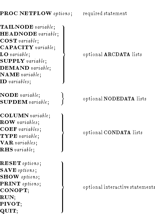
Syntax:
Linear Programming Models: Interior Point algorithm
Below are statements used in PROC NETFLOW, listed
in alphabetical order as they appear in the text that
follows.
- PROC NETFLOW options ;
- CAPACITY variable ;
- COEF variables ;
- COLUMN variable ;
- COST variable ;
- DEMAND variable ;
- ID variables ;
- LO variable ;
- NAME variable ;
- PRINT options ;
- QUIT;
- RESET options ;
- ROW variables ;
- RHS variables ;
- RUN;
- SAVE options ;
- TYPE variable ;
- VAR variables ;
Copyright © 1999 by SAS Institute Inc., Cary, NC, USA. All rights reserved.