Creating a One-Sided Cusum Chart with a Decision Interval

XCHART Statement

Creating a One-Sided Cusum Chart with a Decision Interval

See CUSONES1 in the SAS/QC Sample Library

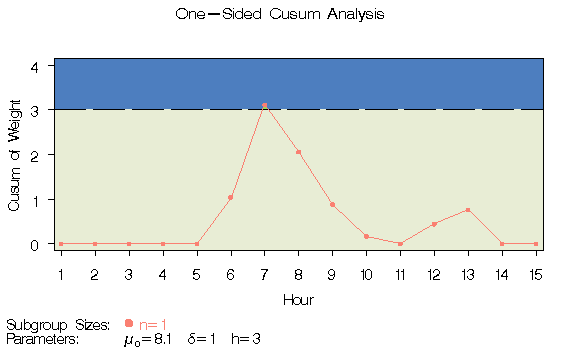
An alternative to the V-mask cusum chart is the one-sided cusum chart with a decision interval, which is sometimes referred to as the "computational form of the cusum chart." This example illustrates how you can create a one-sided cusum chart for individual measurements.

A can of oil is selected every hour for fifteen hours. The cans are weighed, and their weights are saved in a SAS data set named CANS:^*

   data cans;
      length comment $16;
      label hour = 'Hour';
      input hour weight comment $16. ;
      datalines;
    1  8.024
    2  7.971
    3  8.125
    4  8.123
    5  8.068
    6  8.177  Pump Adjusted
    7  8.229  Pump Adjusted
    8  8.072
    9  8.066
   10  8.089
   11  8.058
   12  8.147
   13  8.141
   14  8.047
   15  8.125
   ;

Suppose the problem is to detect a positive shift in the process mean of one standard deviation ( $\delta=1$ ) from the target of 8.100 ounces. Furthermore, suppose that

a known value $\sigma_{0}=0.050$ is available for the process standard deviation
an in-control average run length (ARL) of approximately 100 is required
an ARL of approximately five is appropriate for detecting the shift

Table 12.18 indicates that these ARLs can be achieved with the decision interval h=3 and the reference value k=0.5. The following statements use these parameters to create the chart and tabulate the cusum scheme:

   title "One-Sided Cusum Analysis";
   proc cusum data=cans;
      xchart weight*hour /
         mu0      = 8.100     /* target mean for process     */
         sigma0   = 0.050     /* known standard deviation    */
         delta    = 1         /* shift to be detected        */
         h        = 3         /* cusum parameter h           */
         k        = 0.5       /* cusum parameter k           */
         scheme   = onesided  /* one-sided decision interval */
         tableall             /* table                       */
         cinfill  = ywh      
         cframe   = bigb
         cout     = salmon
         cconnect = salmon
         climits  = black
         coutfill = bilg;
      label weight = 'Cusum of Weight';
   run;

The chart is shown in Figure 12.5.

Figure 12.5: One-Sided Cusum Chart with Decision Interval

The cusum plotted at HOUR=t is

S_t = max(0,S_t-1+(z_t-k))

where S₀=0, and z_t is the standardized deviation of the t^th measurement from the target.

$z_{t} = \frac{ x_{t} - \mu_{0} }{ \sigma_{0} }$

The cusum S_t is referred to as an upper cumulative sum. A shift is signaled at the seventh hour since S₇ exceeds h. For further details, see "One-Sided Cusum Schemes" .

The option TABLEALL requests the tables shown in Figure 12.6, Figure 12.7, and Figure 12.8. The table in Figure 12.6 summarizes the cusum scheme, and it confirms that an in-control ARL of 117.6 and an ARL of 6.4 at $\delta=1$ are achieved with the specified h and k.

One-Sided Cusum Analysis

The CUSUM Procedure

Cusum Parameters
Process Variable	weight (Cusum of Weight)
Subgroup Variable	hour (Hour)
Scheme	One-Sided
Target Mean (Mu0)	8.1
Sigma0	0.05
Delta	1
Nominal Sample Size	1
h	3
k	0.5
Average Run Length (Delta)	6.40390895
Average Run Length (0)	117.595692

Figure 12.6: Summary Table

The table in Figure 12.7 tabulates the information displayed in Figure 12.5.

The CUSUM Procedure

Cumulative Sum Chart Summary for weight
hour	Subgroup Sample Size	Individual Value	Cusum	Decision Interval	Decision Interval Exceeded
1	1	8.0240000	0.0000000	3.0000
2	1	7.9710000	0.0000000	3.0000
3	1	8.1250000	0.0000000	3.0000
4	1	8.1230000	0.0000000	3.0000
5	1	8.0680000	0.0000000	3.0000
6	1	8.1770000	1.0400000	3.0000
7	1	8.2290000	3.1200000	3.0000	Upper
8	1	8.0720000	2.0600000	3.0000
9	1	8.0660000	0.8800000	3.0000
10	1	8.0890000	0.1600000	3.0000
11	1	8.0580000	0.0000000	3.0000
12	1	8.1470000	0.4400000	3.0000
13	1	8.1410000	0.7600000	3.0000
14	1	8.0470000	0.0000000	3.0000
15	1	8.1250000	0.0000000	3.0000

Figure 12.7: Tabulation of One-Sided Chart

The table in Figure 12.8 presents the computational form of the cusum scheme described by Lucas (1976).

The CUSUM Procedure

Computational Cumulative Sum for weight
hour	Subgroup Sample Size	Individual Value	Upper Cusum	Number of Consecutive Upper Sums > 0
1	1	8.0240000	0.0000000	0
2	1	7.9710000	0.0000000	0
3	1	8.1250000	0.0000000	0
4	1	8.1230000	0.0000000	0
5	1	8.0680000	0.0000000	0
6	1	8.1770000	1.0400000	1
7	1	8.2290000	3.1200000	2
8	1	8.0720000	2.0600000	3
9	1	8.0660000	0.8800000	4
10	1	8.0890000	0.1600000	5
11	1	8.0580000	0.0000000	0
12	1	8.1470000	0.4400000	1
13	1	8.1410000	0.7600000	2
14	1	8.0470000	0.0000000	0
15	1	8.1250000	0.0000000	0

Figure 12.8: Computational Form of Cusum Scheme

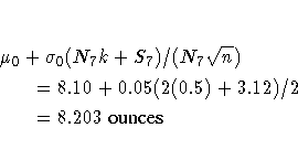
Following the method of Lucas (1976), the process average at the out-of-control point (HOUR=7) can be estimated as

$eqn{\mu_{0} + \sigma_{0} (N_{7}k + S_{7})/ (N_{7} \sqrt{n})} \ & & = 8.10 + 0.05( 2(0.5)+ 3.12) / 2 \ & & = 8.203 { ounces}\;$

where S₇ =3.12 is the upper sum at HOUR=7, and N₇ =2 is the number of successive positive upper sums at HOUR=7.

Chapter Contents
Previous
Next
Top