Lognormal Analysis with Arbitrary Censoring

The RELIABILITY Procedure

Lognormal Analysis with Arbitrary Censoring

This example illustrates analyzing data that have more general censoring than in the previous example. The data can be a combination of exact failure times, left censored, right censored, and interval censored data. The intervals can be overlapping, unlike in the previous exmaple, where the interval endpoints had to be the same for all units.

Table 30.2 shows data from Nelson (1982, p. 409), analyzed by Meeker and Escobar (1998, p. 135). Each of 435 turbine wheels was inspected once to determine whether a crack had developed in the wheel or not. The inspection time (in 100s of hours), the number inspected at the time that had cracked, and the number not cracked are shown in the table. The quantity of interest is the time for a crack to develop.

Table 30.2: Turbine Wheel Cracking Data

Inspection Time	Number	Number
(100 hours)	Cracked	Not Cracked
4	0	39
10	4	49
14	2	31
18	7	66
22	5	25
26	9	30
30	9	33
34	6	7
38	22	12
42	21	19
46	21	15

These data consist only of left and right censored lifetimes. If a unit has developed a crack at an inspection time, the unit is left-censored at the time; if a unit has not developed a crack, it is right-censored at the time. For example, there are 4 left-censored lifetimes and 49 right-censored lifetimes at 1000 hours.

The following statements create a SAS data set named TURBINE thet contains the data in the format necessary for analysis by the RELIABILITY procedure.

   data turbine;                                      
      label t1 = 'Time of Cracking (Hours x 100 )';   
      input t1 t2 f;                                  
      datalines;                                      
   .   4  0                                           
   4   .  39                                          
   .  10  4                                           
   10  .  49                                          
   .  14  2                                           
   14  .  31                                          
   .  18  7                                           
   18  .  66                                          
   .  22  5                                           
   22  .  25                                          
   .  26  9                                           
   26  .  30                                          
   .  30  9                                           
   30  .  33                                          
   .  34  6                                           
   34  .  7                                           
   .  38  22                                          
   38  .  12                                          
   .  42  21                                          
   42  .  19                                          
   .  46  21                                          
   46  .  15                                          
   ;                                                  
   run;

The variables T1 and T2 represent the inspection times and determine whether the observation is right or left censored. If T1 is missing (.), then T2 represents a left-censoring time; if T2 is missing, T1 represents a right-censoring time. The variable F is the number of units that were found to be cracked for left-censored observations, or not cracked for right-censored observations at an inspection time.

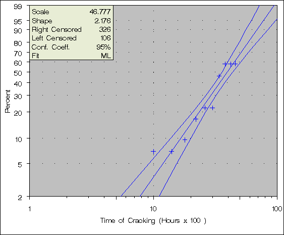
The following statements use the RELIABILITY procedure to produce the probability plot in Figure 30.11 for the data in the data set TURBINE.

   proc reliability data = turbine;      
      distribution lognormal;              
      freq f;                            
      pplot ( t1 t2 ) / maxitem = 5000                          
                        ppout 
                        cframe = ligr;
      inset / ctext = black 
              cfill = ywh;                                                   
      run;

The DISTRIBUTION statement specifies that a lognormal probability plot be created. The FREQ statement identifies the frequency variable F. The option MAXITEM = 5000 specifies that the iterative algorithm that computes the points on the probability plot can take a maximum of 5000 iterations. The algorithm does not converge for this data in the default 1000 iterations, so the maximum number of iterations needs to be increased for convergence. The option PPOUT specifies that a table of the cumulative probabilities plotted on the probability plot be printed, along with standard errors and confidence limits.

The tabular output for the maximum likelihood lognormal fit for this data is shown in Figure 30.12. Figure 30.11 shows the resulting lognormal probability plot with the computed cumulative probability estimates and the lognormal fit line.

Figure 30.11: Lognormal Probability Plot for the Turbine Wheel Data

The RELIABILITY Procedure

Model Information
Input Data Set	WORK.TURBINE
Analysis Variable	t1	Time of Cracking (Hours x 100 )
Analysis Variable	t2
Frequency Variable	f
Distribution	Lognormal (Base e)
Estimation Method	Maximum Likelihood
Confidence Coefficient	95%
Observations Used	21

Cumulative Probability Estimates
Lower Lifetime	Upper Lifetime	Cumulative Probability	95% Confidence Limits		Standard Error
Lower Lifetime	Upper Lifetime	Cumulative Probability	Lower	Upper	Standard Error
.	4	0.0000	0.0000	0.0000	0.0000
10	10	0.0698	0.0264	0.1720	0.0337
14	14	0.0698	0.0177	0.2384	0.0473
18	18	0.0959	0.0464	0.1878	0.0345
22	22	0.1667	0.0711	0.3432	0.0680
26	26	0.2222	0.1195	0.3757	0.0657
30	30	0.2222	0.1203	0.3738	0.0650
34	34	0.4615	0.2236	0.7184	0.1383
38	38	0.5809	0.4085	0.7356	0.0865
42	42	0.5809	0.4280	0.7198	0.0766
46	46	0.5836	0.4195	0.7311	0.0822

Algorithm converged.

Summary of Fit
Observations Used	21
Uncensored Values	0
Right Censored Values	326
Left Censored Values	106
Maximum Loglikelihood	-190.7315

Lognormal Parameter Estimates
Parameter	Estimate	Standard Error	Asymptotic Normal
			95% Confidence Limits
			Lower	Upper
Location	3.6999	0.0708	3.5611	3.8387
Scale	0.7199	0.0887	0.5655	0.9165

Other Lognormal Distribution Parameters
Parameter	Value
Mean	52.4062
Mode	24.0870
Median	40.4436

Lognormal Percentile Estimates
Percent	Estimate	Standard Error	Asymptotic Normal
			95% Confidence Limits
			Lower	Upper
0.1	4.37231983	1.01951851	2.76842301	6.9054406
0.2	5.09347486	1.09461144	3.34261991	7.76142271
0.5	6.33192986	1.19697974	4.37145558	9.17162146
1	7.57765033	1.27242136	5.45258925	10.5309206
2	9.22062896	1.3386637	6.93716343	12.2557295
5	12.3765197	1.38876562	9.93311498	15.4209671
10	16.0761538	1.36948098	13.6041296	18.9973729
20	22.0659696	1.31961576	19.6253961	24.8100476
30	27.7267938	1.47014088	24.9900377	30.7632626
40	33.7009724	1.96843699	30.05555	37.7885463
50	40.4435688	2.86475922	35.2010723	46.4668304
60	48.5351649	4.24027828	40.8969785	57.5999087
70	58.992838	6.33960125	47.7887686	72.8236997
80	74.1269152	9.83371315	57.155116	96.1383677
90	101.74587	17.2094871	73.0370064	141.739407
95	132.160114	26.4307611	89.3034472	195.583668
99	215.856127	55.854619	129.989628	358.442964
99.9	374.099407	121.716176	197.716048	707.835138

Figure 30.12: Partial Listing of the Tabular Output for the Turbine Wheel Data

Chapter Contents
Previous
Next
Top