Example 4.3: Comparing Goodness-of-Fit Tests

HISTOGRAM Statement

Example 4.3: Comparing Goodness-of-Fit Tests

See CAPGOF in the SAS/QC Sample Library

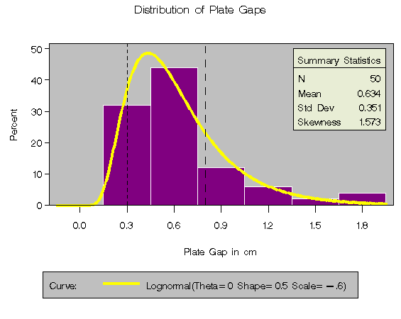
A weakness of the chi-square goodness-of-fit test is its dependence on the choice of histogram midpoints. An advantage of the EDF tests is that they give the same results regardless of the midpoints, as illustrated in this example.

In Example 4.2, the option MIDPOINTS=0.2 TO 1.8 BY 0.2 was used to specify the histogram midpoints for GAP. The following statements refit the lognormal distribution using default midpoints (0.3 to 1.8 by 0.3).

   title1 'Distribution of Plate Gaps';
   legend1 frame cframe=ligr cborder=black position=center;
   proc capability data=plates noprint;
      var gap;
      specs  lsl = 0.3 llsl = 2  clsl=black
             usl = 0.8 lusl = 20 cusl=black;
      histogram /
         lognormal (l=1  color=yellow w=3)
         nospeclegend
         vaxis  = axis1
         legend = legend1
         cfill  = purple
         cframe = ligr;
      inset n mean(5.3) std='Std Dev'(5.3) skewness(5.3) /
         header = 'Summary Statistics' cfill = blank
         pos    = ne
         cfill  = blank;
      axis1  label=(a=90 r=0);
   run;

The histogram is shown in Output 4.3.1.

Output 4.3.1: Lognormal Curve Fit with Default Midpoints

A summary of the lognormal fit is shown in Output 4.3.2. The p-value for the chi-square goodness-of-fit test is 0.0822. Since this value is less than 0.10 (a typical cutoff level), the conclusion is that the lognormal distribution is not an appropriate model for the data. This is the opposite conclusion drawn from the chi-square test in Example 4.2, which is based on a different set of midpoints and has a p-value of 0.2756 (see Output 4.2.2). Moreover, the results of the EDF goodness-of-fit tests are the same since these tests do not depend on the midpoints. When available, the EDF tests provide more powerful alternatives to the chi-square test. For a thorough discussion of EDF tests, refer to D'Agostino and Stephens (1986).

Output 4.3.2: Printed Output for the Lognormal Curve

Distribution of Plate Gaps

The CAPABILITY Procedure

Fitted Lognormal Distribution for gap

Parameters for Lognormal Distribution
Parameter	Symbol	Estimate
Threshold	Theta	0
Scale	Zeta	-0.58375
Shape	Sigma	0.499546
Mean		0.631932
Std Dev		0.336436

Goodness-of-Fit Tests for Lognormal Distribution
Test	Statistic		DF	p Value
Kolmogorov-Smirnov	D	0.06441431		Pr > D	>0.150
Cramer-von Mises	W-Sq	0.02823022		Pr > W-Sq	>0.500
Anderson-Darling	A-Sq	0.24308402		Pr > A-Sq	>0.500
Chi-Square	Chi-Sq	6.69789360	3	Pr > Chi-Sq	0.082

Chapter Contents
Previous
Next
Top