Displaying Stratification in Blocks of Observations

Graphical Enhancements

Displaying Stratification in Blocks of Observations

See SHWBLK in the SAS/QC Sample Library

To display process data stratified into blocks of consecutive observations, specify one or more block-variables in parentheses after the subgroup-variable in the chart statement. The procedure displays a legend identifying blocks of consecutive observations with identical values of the block-variables. The legend displays one track of values for each block-variable. The values are the formatted values of the block-variable. For example, Figure 47.2 displays a legend with a single track for MACHINE, while Figure 47.3 displays a legend with two tracks corresponding to MACHINE and DAY. You can label the tracks themselves by using the LABEL statement to associate labels with the corresponding block-variables; see Figure 47.4 for an illustration.

By default, the legend is placed above the chart as in Figure 47.2. You can control the position of the legend with the BLOCKPOS= option and the position of the legend labels with the BLOCKLABELPOS= option. See the entries in Chapter 46, "Dictionary of Options," as well as the following examples.

The block-variables must be variables in the input data set (a DATA=, HISTORY=, or TABLE= data set). If the input data set is a DATA= data set that contains multiple observations with the same value of the subgroup-variable, the values of a block-variable must be the same for all observations with the same value of the subgroup-variable. In other words, subgroups must be nested within groups determined by block-variables. 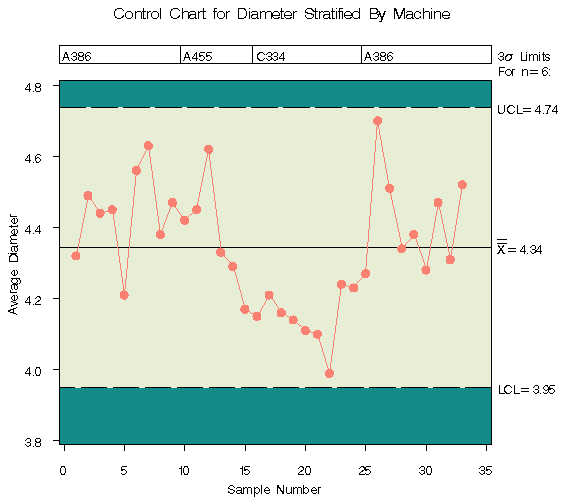The following statements create an $\bar{X}$ chart for the data in PARTS stratified by the block-variable MACHINE. The chart is shown in Figure 47.2.

   title 'Control Chart for Diameter Stratified By Machine';
   symbol v=dot c=salmon;
   proc shewhart history=parts;
      xchart diam*sample (machine) / stddeviations
                                     cframe    = vibg
                                     cinfill   = ywh
                                     cconnect  = salmon;
      label sample = 'Sample Number'
            diamx  = 'Average Diameter' ;
   run;

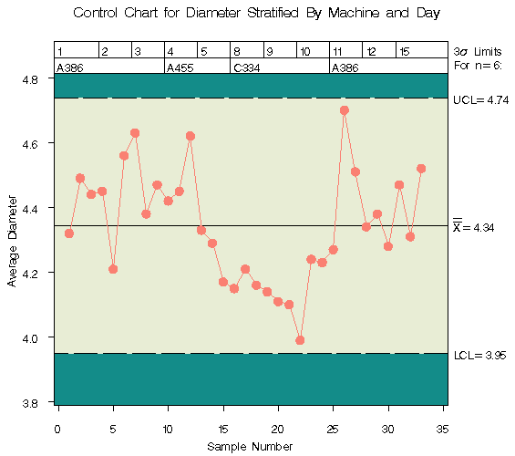
The unique consecutive values of MACHINE (A386, A455, C334, and A386) are displayed in a track above the chart, and they indicate the same relationship between part diameter and machine as the previous example. Note that the track is not labeled (as in Figure 47.4), since no label is associated with MACHINE. A LABEL statement is used to provide labels for the axes.

Figure 47.2: Stratified Control Chart Using a Single Block Variable

Multiple block variables. You can use multiple block-variables to study more than one classification factor with the same chart. The following statements create an $\bar{X}$ chart for the data in PARTS, with MACHINE and DAY as block-variables:

   title 'Control Chart for Diameter Stratified By Machine and Day';
   symbol v=dot c=salmon;
   proc shewhart history=parts;
      xchart diam*sample (machine day) / stddeviations
                                         nolegend
                                         blockpos = 2
                                         cframe   = vibg
                                         cconnect = salmon
                                         cinfill  = ywh;
      label sample = 'Sample Number'
            diamx  = 'Average Diameter' ;
   run;

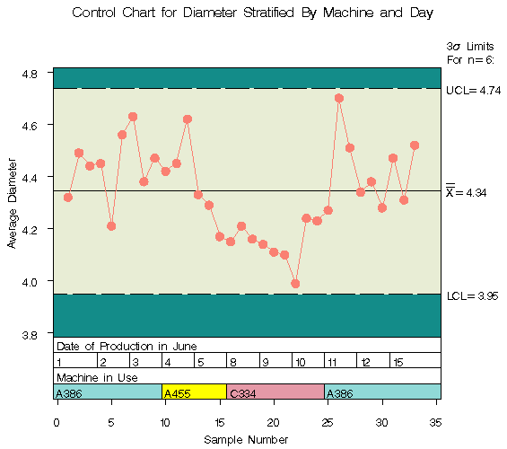
The chart is displayed in Figure 47.3. Specifying BLOCKPOS=2 displays the block-variable legend immediately above the chart, without the gap shown in Figure 47.2. The NOLEGEND option suppresses the sample size legend that appears in the lower left of Figure 47.2.

Figure 47.3: Stratified Control Chart Using Multiple Block Variables

Color fills for legend. You can use the CBLOCKVAR= option to fill the legend track sections with colors corresponding to the values of the block-variables. Provide the colors as values of variables specified with the CBLOCKVAR= option. These variables must be defined as character variables of length 8. The procedure matches the color variables with the block-variables in the order specified. Each section is filled with the color for the first observation in the block. For example, the following statements produce an $\bar{X}$ chart using a color variable named CMACHINE to fill the legend for the block-variable MACHINE:

   data parts2;
      length cmachine $8;
      set parts;
      if      machine='A386' then cmachine='vlibg' ;
      else if machine='A455' then cmachine='yellow' ;
      else if machine='C334' then cmachine='lipk';
      else                        cmachine='white' ;

   proc shewhart history=parts2;
      xchart diam*sample (machine day) / stddeviations
                                         nolegend
                                         blockpos  = 3
                                         cblockvar = cmachine
                                         cframe    = vibg
                                         cconnect  = salmon
                                         cinfill   = ywh;
      label sample  = 'Sample Number'
            diamx   = 'Average Diameter'
            day     = 'Date of Production in June'
            machine = 'Machine in Use';
   run;

Figure 47.4: Color Fill for Block-Variable Legend

The sections for Machine A386 are filled with light gray, the section for Machine A455 is filled with medium gray, and the section for Machine C334 is left white. The legend track for DAY is not filled, since a second color variable was not specified with the CBLOCKVAR= option. Specifying BLOCKPOS=3 positions the legend at the bottom of the chart and facilitates comparison with the subgroup axis. The LABEL statement is used to label the tracks with the labels associated with the block-variables.

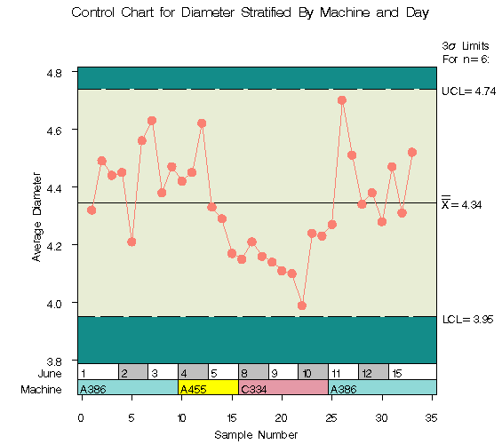
The following statements produce an $\bar{X}$ chart in which both legend tracks are filled:

   data parts3;
      length cday $8;
      set parts2;
      if      day='01' then cday='white';
      else if day='02' then cday='ligr' ;
      else if day='03' then cday='white' ;
      else if day='04' then cday='ligr';
      else if day='05' then cday='white' ;
      else if day='08' then cday='ligr' ;
      else if day='09' then cday='white';
      else if day='10' then cday='ligr' ;
      else if day='11' then cday='white' ;
      else if day='12' then cday='ligr';
      else if day='15' then cday='white' ;
      else                  cday='ligr';

   proc shewhart history=parts3;
      xchart diam*sample (machine day) /
         stddeviations
         nolegend
         ltmargin      = 5
         blockpos      = 3
         blocklabelpos = left
         cblockvar     = (cmachine cday)
         cframe        = vibg
         cconnect      = salmon
         cinfill       = ywh;
      label sample     = 'Sample Number'
            diamx      = 'Average Diameter'
            day        = 'June'
            machine    = 'Machine';
   run;

The chart is displayed in Figure 47.5. The color values of CMACHINE are used to fill the track for MACHINE, and the color values of CDAY are used to fill the track for DAY. Specifying BLOCKLABELPOS=LEFT displays the block variable labels to the left of the block legend. The LTMARGIN= option provides extra space in the left margin to accommodate the label Machine.

Figure 47.5: Stratified Control Chart Using Multiple Block Variables

Chapter Contents
Previous
Next
Top