Calculating the Chart Statistic

Specialized Control Charts

Calculating the Chart Statistic

In this situation, it was shown by Gnanadesikan and Kettenring (1972), using a result of Wilks (1962), that T²_i is exactly distributed as a multiple of a variable with a beta distribution. Specifically,

$T^2_i \sim \frac{(n-1)^2}n B ( \frac{p}2, \frac{n-p-1}2 )$

Tracy, Young, and Mason (1992) used this result to derive initial control limits for a multivariate chart based on three quality measures from a chemical process in the start-up phase: percent of impurities, temperature, and concentration. The remainder of this section describes the construction of a multivariate control chart using their data, which are given here by the data set STARTUP.

   data startup;
      input sample impure temp conc;
      label sample = 'Sample Number'
            impure = 'Impurities'
            temp   = 'Temperature'
            conc   = 'Concentration' ;
      datalines;
    1  14.92  85.77  42.26
    2  16.90  83.77  43.44
    3  17.38  84.46  42.74
    4  16.90  86.27  43.60
    5  16.92  85.23  43.18
    6  16.71  83.81  43.72
    7  17.07  86.08  43.33
    8  16.93  85.85  43.41
    9  16.71  85.73  43.28
   10  16.88  86.27  42.59
   11  16.73  83.46  44.00
   12  17.07  85.81  42.78
   13  17.60  85.92  43.11
   14  16.90  84.23  43.48
   ;

In preparation for the computation of the control limits, the sample size is calculated and parameter variables are defined.

   proc means data=startup noprint ;
      var impure temp conc;
      output out=means n=n;

   data startup;
      if _n_ = 1 then set means;
      set startup;
      p        = 3;
      _subn_   = 1;
      _limitn_ = 1;

Next, the PRINCOMP procedure is used to compute the principal components of the variables and save them in an output data set named PRIN.

   proc princomp data=startup out=prin outstat=scores std cov;
      var impure temp conc;
   run;

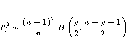
The following statements compute T²_i and its exact control limits, using the fact that T²_i is the sum of squares of the principal components.^* Note that these statements create several special SAS variables so that the data set PRIN can subsequently be read as a TABLE= input data set by the SHEWHART procedure. These special variables begin and end with an underscore character. The data set PRIN is listed in Figure 49.30.

   data prin (rename=(tsquare=_subx_));
      length _var_ $ 8 ;
      drop prin1 prin2 prin3 _type_ _freq_;
      set prin;
      comp1   = prin1*prin1;
      comp2   = prin2*prin2;
      comp3   = prin3*prin3;
      tsquare = comp1 + comp2 + comp3;
      _var_   = 'tsquare';
      _alpha_ = 0.05;
      _lclx_  = ((n-1)*(n-1)/n)*betainv(_alpha_/2, p/2, (n-p-1)/2);
      _mean_  = ((n-1)*(n-1)/n)*betainv(0.5, p/2, (n-p-1)/2);
      _uclx_  = ((n-1)*(n-1)/n)*betainv(1-_alpha_/2, p/2, (n-p-1)/2);
      label tsquare = 'T Squared'
            comp1   = 'Comp 1'
            comp2   = 'Comp 2'
            comp3   = 'Comp 3';
   run;

T2 Chart For Chemical Example

_var_	n	sample	impure	temp	conc	p	_subn_	_limitn_	comp1	comp2	comp3	_subx_	_alpha_	_lclx_	_mean_	_uclx_
tsquare	14	1	14.92	85.77	42.26	3	1	1	0.79603	10.1137	0.01606	10.9257	0.05	0.24604	2.44144	7.13966
tsquare	14	2	16.90	83.77	43.44	3	1	1	1.84804	0.0162	0.17681	2.0410	0.05	0.24604	2.44144	7.13966
tsquare	14	3	17.38	84.46	42.74	3	1	1	0.33397	0.1538	5.09491	5.5827	0.05	0.24604	2.44144	7.13966
tsquare	14	4	16.90	86.27	43.60	3	1	1	0.77286	0.3289	2.76215	3.8640	0.05	0.24604	2.44144	7.13966
tsquare	14	5	16.92	85.23	43.18	3	1	1	0.00147	0.0165	0.01919	0.0372	0.05	0.24604	2.44144	7.13966
tsquare	14	6	16.71	83.81	43.72	3	1	1	1.91534	0.0645	0.27362	2.2534	0.05	0.24604	2.44144	7.13966
tsquare	14	7	17.07	86.08	43.33	3	1	1	0.58596	0.4079	0.44146	1.4354	0.05	0.24604	2.44144	7.13966
tsquare	14	8	16.93	85.85	43.41	3	1	1	0.29543	0.1729	0.73939	1.2077	0.05	0.24604	2.44144	7.13966
tsquare	14	9	16.71	85.73	43.28	3	1	1	0.23166	0.0001	0.44483	0.6766	0.05	0.24604	2.44144	7.13966
tsquare	14	10	16.88	86.27	42.59	3	1	1	1.30518	0.0004	0.86364	2.1692	0.05	0.24604	2.44144	7.13966
tsquare	14	11	16.73	83.46	44.00	3	1	1	3.15791	0.0274	0.98639	4.1717	0.05	0.24604	2.44144	7.13966
tsquare	14	12	17.07	85.81	42.78	3	1	1	0.43819	0.0823	0.87976	1.4003	0.05	0.24604	2.44144	7.13966
tsquare	14	13	17.60	85.92	43.11	3	1	1	0.41494	1.6153	0.30167	2.3320	0.05	0.24604	2.44144	7.13966
tsquare	14	14	16.90	84.23	43.48	3	1	1	0.90302	0.0001	0.00010	0.9032	0.05	0.24604	2.44144	7.13966

Figure 49.30: The Data Set PRIN

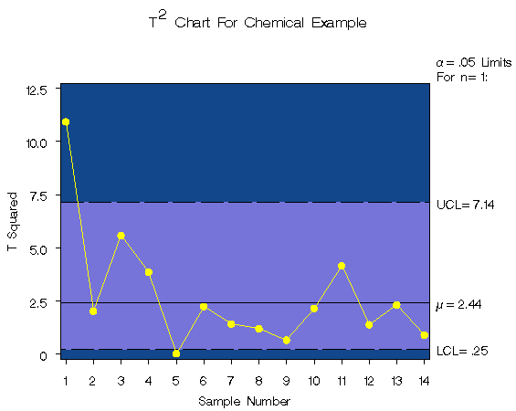
You can now use the data set PRIN as input to the SHEWHART procedure to create the multivariate control chart displayed in Figure 49.31.

   symbol v=dot c=yellow;
   title 'T' m=(+0,+0.5) '2'
             m=(+0,-0.5) ' Chart For Chemical Example';
   proc shewhart table=prin;
      xchart tsquare*sample /
         xsymbol  = mu
         cframe   = vigb
         cinfill  = vlib
         cconnect = yellow
         nolegend ;
   run;

Figure 49.31: Multivariate Control Chart for Chemical Process

The methods used in this example easily generalize to other types of multivariate control charts. You can create charts using the $\chi^2$ and F distributions by using the appropriate CINV or FINV function in place of the BETAINV function in the statements . For details, refer to Alt (1985), Jackson (1980, 1991), and Ryan (1989).

Chapter Contents
Previous
Next
Top