Creating Lognormal Probability Plots

PROBPLOT Statement

Creating Lognormal Probability Plots

See CAPPROB3 in the SAS/QC Sample Library

When you request a lognormal probability plot, you must specify the shape parameter $\sigma$ for the lognormal distribution (see Table 9.13 for the equation). The value of $\sigma$ must be positive, and typical values of $\sigma$ range from 0.1 to 1.0. Alternatively, you can specify that $\sigma$ is to be estimated from the data.

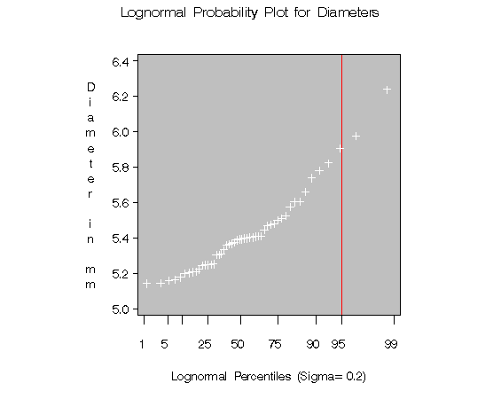
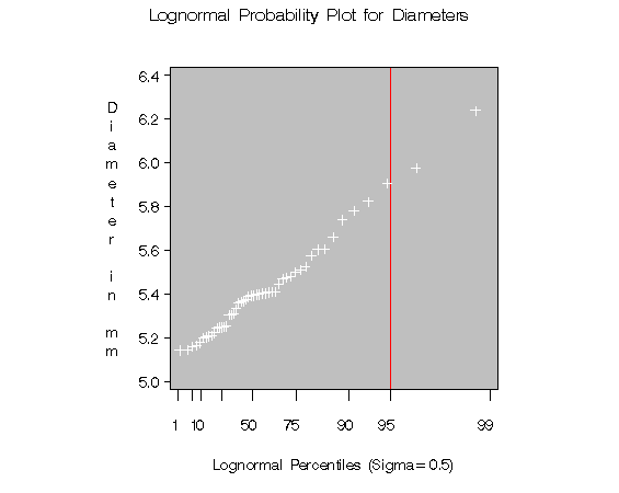
The following statements illustrate the first approach by creating a series of three lognormal probability plots for the variable DIAMETER introduced in the preceding example:

title 'Lognormal Probability Plot for Diameters';
proc capability data=measures noprint;
   probplot diameter / lognormal(sigma=0.2 0.5 0.8
                                 color=yellow)
                       HREF=95
                       lHREF=1
                       square
                       cHREF=red
                       cframe = ligr;
run;

The LOGNORMAL option requests plots based on the lognormal family of distributions, and the SIGMA= option requests plots for $\sigma$ equal to 0.2, 0.5, and 0.8. These plots are displayed in Figure 9.3, Figure 9.4, and Figure 9.5, respectively. The value $\sigma=0.5$ in Figure 9.4 produces the most linear pattern.

The SQUARE option displays the probability plot in a square format, the HREF=option requests a reference line at the 95^th percentile, and the LHREF=option specifies the line type for the reference line.

Figure 9.3: Probability Plot Based on Lognormal Distribution with $\sigma=0.2$

Figure 9.4: Probability Plot Based on Lognormal Distribution with $\sigma=0.5$

Figure 9.5: Probability Plot Based on Lognormal Distribution with $\sigma=0.8$

Based on Figure 9.4, the 95^th percentile of the diameter distribution is approximately 5.9 mm, since this is the value corresponding to the intersection of the point pattern with the reference line.

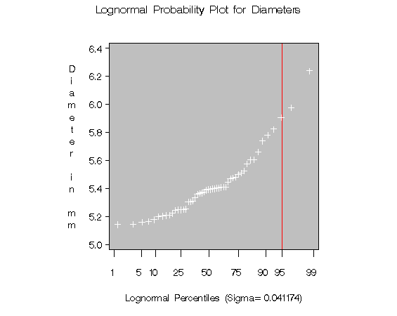
The following statements illustrate how you can create a lognormal probability plot for DIAMETER using a local maximum likelihood estimate for $\sigma$ .

title 'Lognormal Probability Plot for Diameters';
proc capability data=measures noprint;
   probplot diameter / lognormal(sigma=est
                                 color=yellow)
                       HREF=95
                       lHREF=1
                       square
                       cHREF=red
                       cframe = ligr;
run;

The plot is displayed in Figure 9.6. Note that the maximum likelihood estimate of $\sigma$ (in this case 0.041) does not necessarily produce the most linear point pattern. This example is continued in Example 9.2.

Figure 9.6: Probability Plot Based on Lognormal Distribution with Estimated $\sigma$

Chapter Contents
Previous
Next
Top