Parameter Estimates and Associated Statistics

Chapter Contents

Introduction to Regression Procedures

Parameter Estimates and Associated Statistics

Parameter estimates are formed using least-squares criteria by solving the normal equations

(X' X)b = X' y

for the parameter estimates b, yielding

b = (X'X)^-1X'y

Assume for the present that (X'X) is full rank (this assumption is relaxed later). The variance of the error $\sigma^2$ is estimated by the mean square error

$s^2 = {MSE} = \frac{SSE}{n-k} = \frac{1}{n-k}\sum_{i=1}^n ( y_i - x_i b )^2$

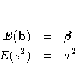
where x_i is the ith row of regressors. The parameter estimates are unbiased:

$E (b) & = & {{\beta}} \E (s^2) & = & \sigma^2$

The covariance matrix of the estimates is

${VAR} (b) = (X^' X)^{-1} \sigma^2$

The estimate of the covariance matrix is obtained by replacing $\sigma^2$ with its estimate, s², in the formula preceding:

COVB = (X' X)^-1 s²

The correlations of the estimates are derived by scaling to 1s on the diagonal.

Let

$S & = & {diag} ( (X^' X)^{-1} )^{-\frac{1}2} \{CORRB} & = & S ( X^' X )^{-1} S$

Standard errors of the estimates are computed using the equation

${STDERR}(b_i) = \sqrt{ (X^' X)^{-1}_{ii} s^2 }$

where (X' X)^-1_ii is the ith diagonal element of (X' X)^-1. The ratio

t = [(b_i)/( STDERR(b_i))]

is distributed as Student's t under the hypothesis that $\beta_i$ is zero. Regression procedures display the t ratio and the significance probability, which is the probability under the hypothesis $\beta_i=0$ of a larger absolute t value than was actually obtained. When the probability is less than some small level, the event is considered so unlikely that the hypothesis is rejected.

Type I SS and Type II SS measure the contribution of a variable to the reduction in SSE. Type I SS measure the reduction in SSE as that variable is entered into the model in sequence. Type II SS are the increment in SSE that results from removing the variable from the full model. Type II SS are equivalent to the Type III and Type IV SS reported in the GLM procedure. If Type II SS are used in the numerator of an F test, the test is equivalent to the t test for the hypothesis that the parameter is zero. In polynomial models, Type I SS measure the contribution of each polynomial term after it is orthogonalized to the previous terms in the model. The four types of SS are described in Chapter 12, "The Four Types of Estimable Functions."

Standardized estimates are defined as the estimates that result when all variables are standardized to a mean of 0 and a variance of 1. Standardized estimates are computed by multiplying the original estimates by the sample standard deviation of the regressor variable and dividing by the sample standard deviation of the dependent variable.

R² is an indicator of how much of the variation in the data is explained by the model. It is defined as

R² = 1 - [ SSE/ TSS]

where SSE is the sum of squares for error and TSS is the corrected total sum of squares. The Adjusted R² statistic is an alternative to R² that is adjusted for the number of parameters in the model. This is calculated as

ADJRSQ = 1 - [(n - i)/(n - p)] (1 - R² )

where n is the number of observations used to fit the model, p is the number of parameters in the model (including the intercept), and i is 1 if the model includes an intercept term, and 0 otherwise.

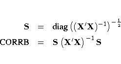
Tolerances and variance inflation factors measure the strength of interrelationships among the regressor variables in the model. If all variables are orthogonal to each other, both tolerance and variance inflation are 1. If a variable is very closely related to other variables, the tolerance goes to 0 and the variance inflation gets very large. Tolerance (TOL) is 1 minus the R² that results from the regression of the other variables in the model on that regressor. Variance inflation (VIF) is the diagonal of (X' X)^-1 if (X' X) is scaled to correlation form. The statistics are related as

VIF = [1/ TOL]

Models Not of Full Rank

If the model is not full rank, then a generalized inverse can be used to solve the normal equations to minimize the SSE:

b = (X' X)^- X' y

However, these estimates are not unique since there are an infinite number of solutions using different generalized inverses. PROC REG and other regression procedures choose a nonzero solution for all variables that are linearly independent of previous variables and a zero solution for other variables. This corresponds to using a generalized inverse in the normal equations, and the expected values of the estimates are the Hermite normal form of X' X multiplied by the true parameters:

$E (b) = (X^' X)^{-} (X^' X) {{\beta}}$

Degrees of freedom for the zeroed estimates are reported as zero. The hypotheses that are not testable have t tests displayed as missing. The message that the model is not full rank includes a display of the relations that exist in the matrix.

Chapter Contents
Previous
Next
Top