Introductory Example

Introduction to Regression Procedures

Introductory Example

Regression analysis is the analysis of the relationship between one variable and another set of variables. The relationship is expressed as an equation that predicts a response variable (also called a dependent variable or criterion) from a function of regressor variables (also called independent variables, predictors, explanatory variables, factors, or carriers) and parameters. The parameters are adjusted so that a measure of fit is optimized. For example, the equation for the ith observation might be

$y_i = \beta_0 + \beta_1 x_i + \epsilon_i$

where y_i is the response variable, x_i is a regressor variable, $\beta_0$ and $\beta_1$ are unknown parameters to be estimated, and $\epsilon_i$ is an error term.

You might use regression analysis to find out how well you can predict a child's weight if you know that child's height. Suppose you collect your data by measuring heights and weights of 19 school children. You want to estimate the intercept $\beta_0$ and the slope $\beta_1$ of a line described by the equation

${Weight} = \beta_0 + \beta_1 {Height} + \epsilon$

where

Weight: is the response variable.
$\beta_0$ , $\beta_1$: are the unknown parameters.
Height: is the regressor variable.
$\epsilon$: is the unknown error.

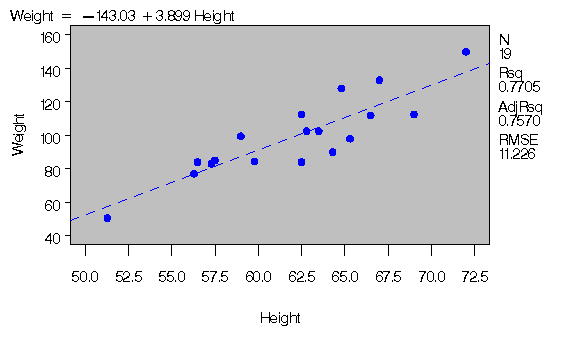
The data are included in the following program. The results are displayed in Figure 3.1 and Figure 3.2.

   data class;
      input Name $ Height Weight Age;
      datalines;
   Alfred  69.0 112.5 14
   Alice   56.5  84.0 13
   Barbara 65.3  98.0 13
   Carol   62.8 102.5 14
   Henry   63.5 102.5 14
   James   57.3  83.0 12
   Jane    59.8  84.5 12
   Janet   62.5 112.5 15
   Jeffrey 62.5  84.0 13
   John    59.0  99.5 12
   Joyce   51.3  50.5 11
   Judy    64.3  90.0 14
   Louise  56.3  77.0 12
   Mary    66.5 112.0 15
   Philip  72.0 150.0 16
   Robert  64.8 128.0 12
   Ronald  67.0 133.0 15
   Thomas  57.5  85.0 11
   William 66.5 112.0 15
   ;
   symbol1 v=dot c=blue height=3.5pct;
   proc reg;
      model Weight=Height;
      plot Weight*Height/cframe=ligr;
   run;

The REG Procedure

Model: MODEL1

Dependent Variable: Weight

Analysis of Variance
Source	DF	Sum of Squares	Mean Square	F Value	Pr > F
Model	1	7193.24912	7193.24912	57.08	<.0001
Error	17	2142.48772	126.02869
Corrected Total	18	9335.73684

Root MSE	11.22625	R-Square	0.7705
Dependent Mean	100.02632	Adj R-Sq	0.7570
Coeff Var	11.22330

Parameter Estimates
Variable	DF	Parameter Estimate	Standard Error	t Value	Pr > \|t\|
Intercept	1	-143.02692	32.27459	-4.43	0.0004
Height	1	3.89903	0.51609	7.55	<.0001

Figure 3.1: Regression for Weight and Height Data

Figure 3.2: Regression for Weight and Height Data

Estimates of $\beta_0$ and $\beta_1$ for these data are b₀=-143.0 and b₁=3.9, so the line is described by the equation

Weight = -143.0 + 3.9* Height

Regression is often used in an exploratory fashion to look for empirical relationships, such as the relationship between Height and Weight. In this example, Height is not the cause of Weight. You would need a controlled experiment to confirm scientifically the relationship. See the "Comments on Interpreting Regression Statistics" section for more information.

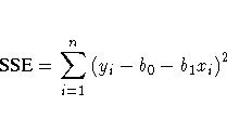
The method most commonly used to estimate the parameters is to minimize the sum of squares of the differences between the actual response value and the value predicted by the equation. The estimates are called least-squares estimates, and the criterion value is called the error sum of squares

${SSE} = \sum_{i=1}^n ( y_i - b_0 - b_1 x_i )^2$

where b₀ and b₁ are the estimates of $\beta_0$ and $\beta_1$ that minimize SSE.

For a general discussion of the theory of least-squares estimation of linear models and its application to regression and analysis of variance, refer to one of the applied regression texts, including Draper and Smith (1981), Daniel and Wood (1980), Johnston (1972), and Weisberg (1985).

SAS/STAT regression procedures produce the following information for a typical regression analysis:

parameter estimates using the least-squares criterion
estimates of the variance of the error term
estimates of the variance or standard deviation of the sampling distribution of the parameter estimates
tests of hypotheses about the parameters

SAS/STAT regression procedures can produce many other specialized diagnostic statistics, including

collinearity diagnostics to measure how strongly regressors are related to other regressors and how this affects the stability and variance of the estimates (REG)
influence diagnostics to measure how each individual observation contributes to determining the parameter estimates, the SSE, and the fitted values (LOGISTIC, REG, RSREG)
lack-of-fit diagnostics that measure the lack of fit of the regression model by comparing the error variance estimate to another pure error variance that is not dependent on the form of the model (CATMOD, PROBIT, RSREG)
diagnostic scatter plots that check the fit of the model and highlighted scatter plots that identify particular observations or groups of observations (REG)
predicted and residual values, and confidence intervals for the mean and for an individual value (GLM, LOGISTIC, REG)
time-series diagnostics for equally spaced time-series data that measure how much errors may be related across neighboring observations. These diagnostics can also measure functional goodness of fit for data sorted by regressor or response variables (REG, SAS/ETS procedures).

Chapter Contents
Previous
Next
Top