
Chapter Contents
![[*]](../../common/images/prev1.gif)
Previous

Next
|
Chapter Contents |
Previous |
Next |
| SAS/INSIGHT Software |
The Confidence Intervals table gives confidence intervals for the mean, standard deviation, and variance for the confidence coefficient specified. You specify the confidence intervals either in the distribution output options dialog or from the Tables menu.
A 100(1-![]() )% confidence interval for the mean
has upper and lower limits
)% confidence interval for the mean
has upper and lower limits
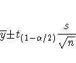
where ![]() is the (1-
is the (1-![]() /2) critical value of the
Student's t-statistic with n-1 degrees of freedom.
/2) critical value of the
Student's t-statistic with n-1 degrees of freedom.
A 100(1-![]() )% confidence interval for the standard deviation
has upper and lower limits
)% confidence interval for the standard deviation
has upper and lower limits
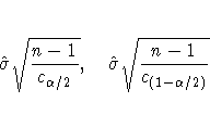
where ![]() and
and ![]() are the
are the ![]() /2 and (1-
/2 and (1-![]() /2) critical values
of the chi-square statistic with n-1 degrees of freedom.
/2) critical values
of the chi-square statistic with n-1 degrees of freedom.
A 100(1-![]() )% confidence interval for the variance
has upper and lower limits equal to the squares of
the corresponding upper and lower limits for the standard deviation.
)% confidence interval for the variance
has upper and lower limits equal to the squares of
the corresponding upper and lower limits for the standard deviation.
Figure 1.7 shows a table of the 95% confidence intervals for mean, standard deviation, and variance.
![[Figure]](images/dist11.gif)
|
The sample standard deviation is a commonly used estimator of the population scale. But the estimate is sensitive to the presence of outliers and may not remain bounded when a single data point is replaced by an arbitrary number. With robust scale estimators, the estimates remain bounded even when a portion of the data points are replaced by arbitrary numbers.
A simple robust scale estimator is the interquartile range,
which is the difference between the upper and lower quartiles.
For a normal population, the standard deviation ![]() can
be estimated by dividing the interquartile range by 1.34898.
can
be estimated by dividing the interquartile range by 1.34898.
Gini's mean difference is also a robust estimator of
the standard deviation ![]() .It is computed as
.It is computed as
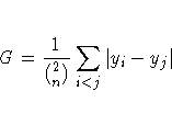
If the observations are from a normal distribution,
then ![]() is an unbiased estimator of
the standard deviation
is an unbiased estimator of
the standard deviation ![]() .A very robust scale estimator is the MAD,
the median absolute deviation about the median (Hampel, 1974.)
.A very robust scale estimator is the MAD,
the median absolute deviation about the median (Hampel, 1974.)
For a normal distribution, 1.4826 MAD can be used to estimate the
standard deviation ![]() .
.
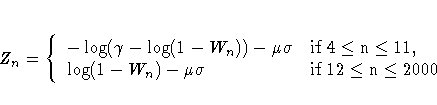
The MAD statistic has low efficient at normal distributions and it may not be appropriate for symmetric distributions. Rousseeuw and Croux (1993) proposed two new statistics as alternatives to the MAD statistic.
The first statistic is Sn,
The other statistic is Qn,
As in Sn, cqnQn is used to
estimate the standard deviation ![]() , where cqnare the correction factors.
, where cqnare the correction factors.
A Robust Measures of Scale table includes
statistics of interquartile range, Gini's mean difference G,
MAD, Qn, and Sn,
with their corresponding estimates of ![]() .
.
![[Figure]](images/dist13.gif)
|
SAS/INSIGHT software provides tests for the null hypothesis that the input data values are a random sample from a normal distribution. These test statistics include the Shapiro-Wilk statistic, W, and statistics based on the empirical distribution function: the Kolmogorov-Smirnov, Cramer-von Mises, and Anderson-Darling statistics.
The Shapiro-Wilk statistic is the ratio of the best estimator of the variance (based on the square of a linear combination of the order statistics) to the usual corrected sum of squares estimator of the variance. W must be greater than zero and less than or equal to one, with small values of W leading to rejection of the null hypothesis of normality. Note that the distribution of W is highly skewed. Seemingly large values of W (such as 0.90) may be considered small and lead to the rejection of the null hypothesis.
The W statistic is computed when the sample size is less than or equal to 2000. When the sample size is greater than three, the coefficients for computing the linear combination of the order statistics are approximated by the method of Royston (1992).
With a sample size of three, the probability distribution of W is known and is used to determine the significance level. When the sample size is greater than three, simulation results are used to obtain the approximate normalizing transformation (Royston, 1992)
The Kolmogorov statistic assesses the discrepancy
between the empirical distribution and the estimated
hypothesized distribution.
For a test of normality, the hypothesized distribution is
a normal distribution function with parameters ![]() and
and
![]() estimated by the sample mean and standard deviation.
The probability of a larger test statistic is obtained
by linear interpolation within the range of simulated
critical values given by Stephens (1974).
estimated by the sample mean and standard deviation.
The probability of a larger test statistic is obtained
by linear interpolation within the range of simulated
critical values given by Stephens (1974).
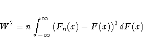
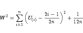
The Cramer-von Mises statistic ( W2) is defined as
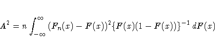
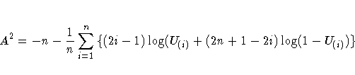
The Anderson-Darling statistic ( A2) is defined as
The probability of a larger test statistic is obtained by linear interpolation within the range of simulated critical values in D'Agostino and Stephens (1986).
A Tests for Normality table includes statistics of Shapiro-Wilk, Kolmogorov, Cramer-von Mises, and Anderson-Darling, with their corresponding p-values.
![[Figure]](images/dist14.gif)
|
|
Chapter Contents |
Previous |
Next |
 Top |
Copyright © 1999 by SAS Insitute Inc., Cary, NC, USA. All rights reserved.