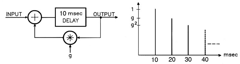
In this diagram, we keep the delay in the
phasing range of 10 ms, and identify the feedback
gain as g. For all values of g
below 1 (expressed with a decimal such as .8 or as the
equivalent percentage, in this case 80%) the repetitions
in the output will fall off either very rapidly, for
instance, with a gain less than 60%, or very slowly with
a gain above 90%. In other words, the decay time is
exponentially dependent on the gain. In systems
theory this is called “negative feedback” which
paradoxically has the positive outcome of keeping the
system stable.
For instance, as noted in the output diagram with the
gain values of g, g2 etc, if the gain is 50%,
the repetitions will fall off as .5, .25, .125, ... and
approach zero very quickly. However, with 90%, they will
fall off as .9, .81, .73, .65, … which is much slower.
A gain factor above 1.0 is called “positive feedback”
which means the repetitions grow exponentially
like inflation, and in the case of audio, will go into
signal saturation (i.e. distortion) fairly
quickly depending on the speed of the repetition delay
and the gain factor. In digital software, it is common
to find the gain factor hard limited to a maximum of 99%
(.99) to avoid this kind of problem.
The analog tradition was more free-wheeling in that it
allowed momentary instances of positive gain to allow a
rapid buildup, likely followed by a decrease below 1 to
avoid saturation and distortion. Digital designers, with
some notable exceptions noted below, are more protective
of their consumers!
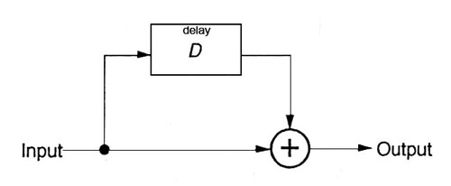
What is the most remarkable about
adding feedback to the circuit is that the frequency
response essentially becomes its opposite, as
can be seen below where the top diagram is the single
delay phasing effect, and the bottom diagram is where
feedback is added:
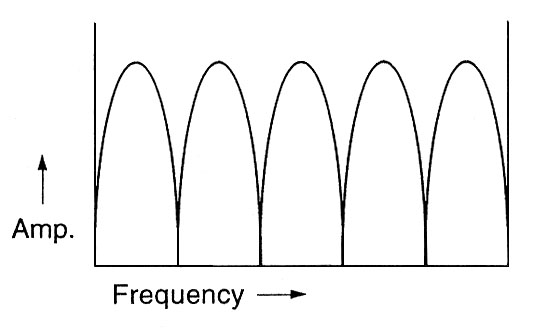
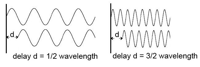
- the narrow notches at the 1/2
wavelength intervals (A, B, C) become broad
regions of attenuation according to the set of odd
harmonic frequencies, 1, 3, 5, ....
- the broad regions of
amplification in between become quite narrow
peaks (a, b, c) , spaced according to the set of
even harmonic frequencies, 2, 4, 6, ....
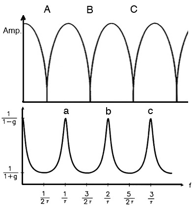
Comb filter frequency response without fee
dback (top) and
with feedback (bottom)
In terms of perception, the “hollow” impression of the
missing frequencies with phasing, becomes potentially
very strong regions of harmonically related spectral
pitches (also known as repetition pitches).
Unsurprisingly, this addition of boosted harmonics to
even a noise spectrum has proved popular with sound
designers and software developers to the extent that
in a comb filter app, this is what you’ll mainly get,
but with typically little information as to why it
works.
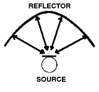
Historical
interlude. It was easy to find
environmental examples of the comb filter effect
with broad-band moving sounds and a strong
reflective surface or building nearby. But can you
think of any purely acoustic situation that
could produce a harmonic pitch impression that was
the result of multiple and equal
reflections? Clearly this is easy to produce
electronically, but acoustically? Answer here, and it’s
very intriguing!
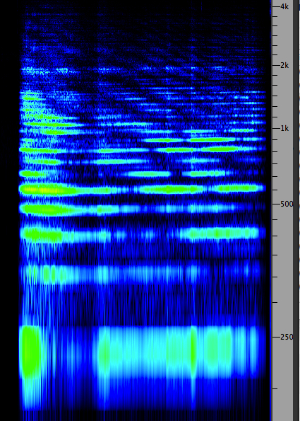
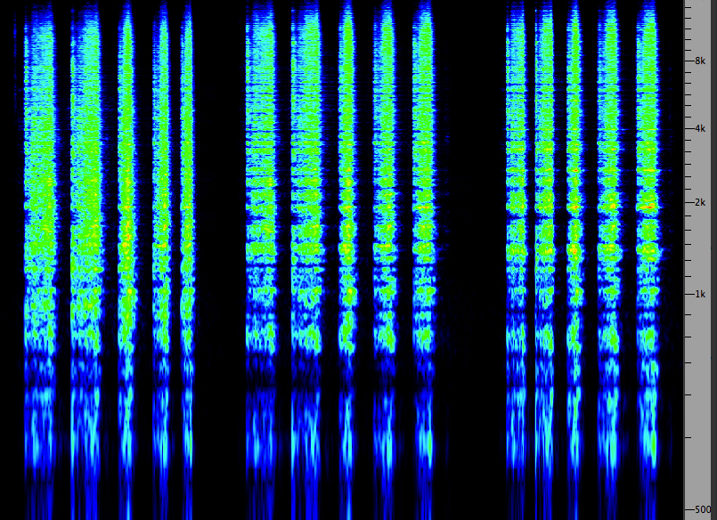
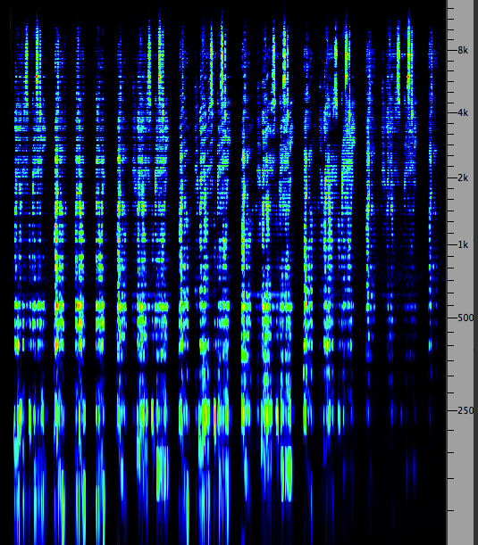
Examples. In the first sound
example below, we hear three sequences: (1) the
original sound of carding wool, which is broadband;
(2) a version with phasing created with about a 1 ms
delay and no feedback; (3) the same with feedback. The
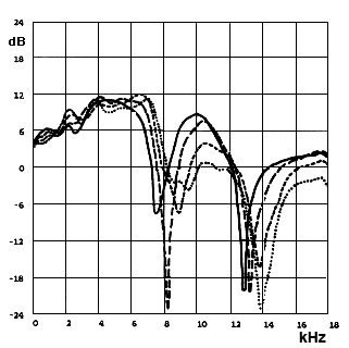
corresponding spectra are shown at the right, with the
characteristic striation in the second
example, and the boosted regions in the third, which
do sound about an octave higher.
Carding wool, original, without
and with feedback
Source:
WSP Can 33 take 1& 2
|
(Click to enlarge)
|
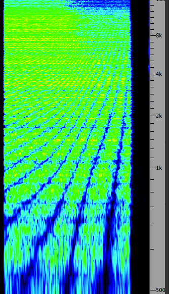
Delays correlated with
amplitude, without and with feedback
|
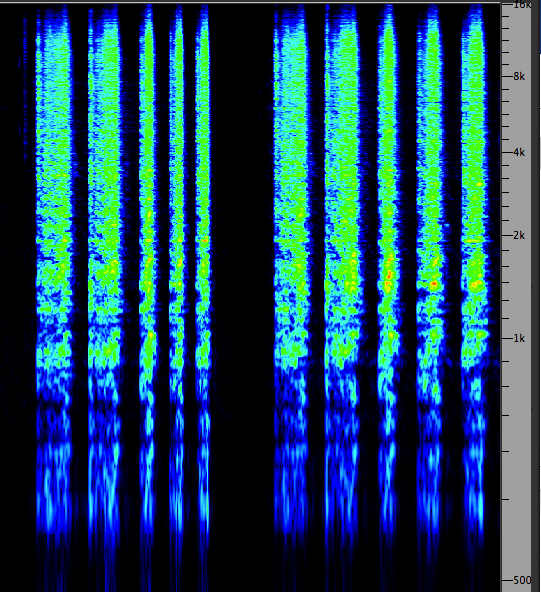
(Click to enlarge)
|
In the second sound example above, we hear the phasing
examples again, without and with feedback, where the
time delays are correlated with the amplitude of
the signal, a type of effect seldom offered in
plug-ins today. These examples were realized with a
Lexicon Digital Delay in hardware that will be
illustrated below. The correlation is that higher
amplitudes are correlated with shorter delays,
hence the sense of rising spectral pitch. Given that
the amplitude also correlated with the manual effort
producing the sound, this example (while abstracted)
does integrate the processing with the actual sound.
This kind of processed delays could
be called a modulation of the delays, but in
the more general case of delay modulation, there is a
periodic repetition of the delay changes
typically controlled by a subaudio oscillator,
where the frequency, depth and waveform of the
modulation will be the control variables, as
illustrated below.
Unfortunately, delay modulation of this type
is often referred to as chorusing, as it sort
of blurs the resulting pitch (or makes it seem very
mechanical like a bad vibrato), and should not be
confused with the acoustic choral
effect created by multiple sound sources
that are slightly detuned and staggered
in their onset, thereby adding volume
(and blend) to the perceived sound (similar to a
musical ensemble).
Index
C. Sources of time delays.
Although acoustically delayed sound in the form of
reflections is ubiquitous, in the early part of the
20th century it proved difficult to create them
electrically. The intent was to produce artificial
reverberation, but that depended on having multiple
delays. The basic problem, both for audio and then the
emerging development of computers, was the lack of memory,
particularly of the read-write variety. How to store
signals and be able, preferably in real time, to
retrieve them?
The history of both the analog and digital
developments is indeed fascinating but beyond our
scope, so let’s go to the two standard methods that
emerged for audio. In the analog domain, the
separation of the recording head from the playback
head in tape
recording was the critical development.
It also improved the performance of each process if
they were separate heads, even though the less
expensive machines for home use generally continued to
keep them as one unit (since what was mainly involved
was to switch the direction of the magnetic process,
to imprint the signal or to extract it).
The three-head tape recorder (which included
an erase head prior to the record and playback
heads) meant there was a physical distance between the
record head (R) and the playback head (P) as shown in
the following diagrams. If this was on average 2
inches or 5 cm, and the standard playback speeds were
7.5 ips (inches/sec) or 19 cm/sec, then the delay
between the recording and the playback would be around
1/4 second. The professional speed of 15 ips (or 38
cm/sec) would result in approximately a 1/8 second
delay. These values were definitely in the range of an
echo for 1/4 sec, and almost approaching the range of
reverberation for 1/8 sec, despite it being a single
repetition.
In the analog recording studio
there emerged a standard set of circuits for
exploiting this phenomenon with stereo
recorders, which can be divided into mono and stereo
versions of the circuit (i.e. one or two inputs,
marked A and B below), with three possible types of
processes:
A. simple echo, i.e. a single
repetition;
B. feedback of the signal back into the
recording head with usually an external gain control
through a mixer to control feedback levels of the
multiple repetitions;
C. echo plus feedback, which is a combination
of the other two, with the delayed echo being fed back
to the opposite channel of the recording, producing a
“ping pong” left to right to left kind of feedback.
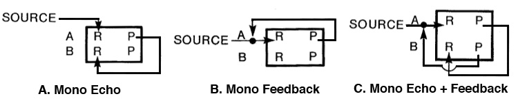
In mono echo, the sound is
recorded on the left channel and a fraction of a
second later is reproduced with a corresponding delay
that is sent to the right channel where it too is
recorded, thereby producing an echo. When a mixer was
involved, the strength of the echo could be
controlled, but otherwise it would implicitly
controlled by the playback and record levels.
In mono feedback, the delayed playback signal
was fed back into the same channel (in this case A).
With a studio mixer this was simply a matter of
controlling the playback level and sending it back to
the recorder. If a mixer wasn’t used, there were
connectors that combined (not mixed, because no levels
were involved) the two signals and you took your
chances on feedback levels unless there was a playback
level control.
In echo plus feedback, both connections are
combined except that the left channel playback is
connected to the right channel, and the right channel
playback is connected back to the left channel,
producing a very attractive pseudo-stereo effect and
the characteristic left-right-left multiple echoes.
Note that the delay for the feedback is twice
that of the echo, as there are now two delays before
the feedback loop is completed. Needless to say, this
was a very popular technique that is often imitated in
digital apps.
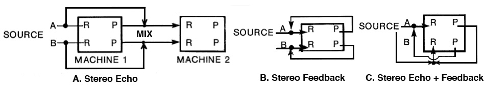
In the stereo vision of these circuits (i.e.
with two inputs) there is an interesting anomaly with
what might be regarded as the simplest circuit, the stereo
echo (with a single repetition). It can’t be
done with a single machine (and is sometimes still
tricky to do in the digital domain). If you were to
connect the delayed playback from either channel to
the opposite, it would produce feedback, and not a
single echo. Therefore it had to be done using two
machines where the second one was used to record the
result.
Stereo feedback is a simple extension of the
mono version, where each playback stays on its own
channel, and the stereo echo plus feedback,
although it looks a bit complex, is simply routing the
delayed playback signals to the opposite channel for
recording (on a mixer this would be simply reversing
the pan knobs so that the signal went to the opposite
channel). Like its mono counterpart, this circuit and
effect was very popular because of the pseudo-stereo
effect.
Footstep
sequence with multiple stereo delays, from Barry
Truax's Soundscape Study (1974)
Source: WSP Can 49, take 8
In
this analog studio use of stereo delays, the source is a
beautifully recorded sequence of a person walking across
a covered bridge in New Brunswick. The microphone is in
the middle, and so there is a very strong left to right
spatial movement created with the footsteps. Instead of
the echo just following the person’s steps, the channels
are reversed so that the illusion is of a second
person walking right to left. To add a more dramatic
element, the echo only starts in the middle
where the steps are closest to the microphone. So, we
are presented with the illusion that one person
approaches, and two people depart!
On the second pass, the footsteps are now echoed right
from the start, and then doubled again in the middle.
This happens over several passes, with the echo density
getting increasingly dense. The original delay
syncopated the rhythm (the footsteps occur at about .5
sec intervals and the delay is .33 sec, making it a 2/3
1/3 triple rhythm), so as a result the echoes quickly
fill in the silences between the steps. The exercise was
designed to reflect Murray Schafer’s comment about
environmental rhythms speeding up from footsteps to
galloping horses to trains and eventually flatline
sounds.
The long and the short of it.
The main limitation of these circuits was the fixed
delay between the record and playback heads, with
only the available tape speeds to choose from
(usually there were only two or three speed options).
One limited variation existed in the form of recording
to a
tape loop (i.e. a piece of tape where its
end is spliced to its beginning) only for the purposes
of recording a delay. To keep some tension on the
loop during playback, it usually was hung vertically
with a small tape reel to keep it taut. If the tape
recorder had a variable speed function, then the delay
could be adjusted by varying the speed of the tape. This
practice became mirrored in the digital domain by a
“looping memory” concept called a delay line
which will be illustrated below.
In order to create very long delays,
particularly with feedback, and very short delays
for phasing, considerable ingenuity had to be used. The
solution for long delays has already been hinted at with
the stereo echo. In the above diagram the connection
between the two machines is purely electrical. But there
is also a physical distance between the machines
that could be varied, or else the path of the tape could
be creatively wound around a separate stand, such that
the tape would travel from the first machine via a
possibly lengthy detour and be played back (only) many
seconds later on the second machine, as shown here.
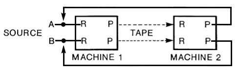
This circuit called delayed feedback, which
always had a large “fun quotient” attached to it in
the analog studio, involved an interesting type of
performability. Now that the feedback loop was many
seconds long, it took awhile for the feedback signal
to enter the mix, and an even longer time for the
feedback levels to stabilize to an overall sound
texture. However, like all feedback circuits with
their exponential behaviour, small changes in
feedback level resulted in significant changes
in the behaviour of the circuit, except that in this
case it took a much longer time for the result to be
heard.
One practical advantage of any feedback circuit in the
analog studio was that a small EQ (e.g. rolling off
the high frequencies that might build up through tape
hiss) only needed a small amount of attenuation
because it would be repeatedly applied with
every feedback loop, and likewise a presence boost in
the 1-4 kHz region could be used to counteract the
inevitable degradation of the analog re-recording
process. In some cases, a more daring or conceptually
oriented user would only use tape hiss as the sole
source material, perhaps to confirm that the medium is
not only the message but its content as well!
A fascinating variation of the long delay feedback
circuit was to perform the entire process with
reversed sound (i.e. playing the source sound in
the backwards direction). Given that analog feedback
went from copies of the original to a denser and
possibly more degraded form, this allowed the
trajectory of the sound to be in the opposite
direction: starting in a dense, degraded form and
gradually transitioning back to the less dense
original. The trick was to perform the feedback levels
while hearing the sounds in their backwards direction.
Then, the process was stopped, and the recorded tape
reversed and only then could you hear what the
forwards version of the material sounded like!
Delayed feedback sequence with an ax hit,
footsteps and closing door, from Barry Truax's Soundscape
Study (1974)
Source: WSP Can 85, take 7
Lastly, how could the extremely
small time delays involved in phasing (i.e. less
than 10 ms) be achieved with analog recorders? Here’s a
hint: unlike digital recorders, the actual playback
speed of an analog recorder, even when well calibrated,
was never exactly the same. In early models, even the
varying weight of the source and take-up reels during
playback, for instance, might affect the speed of the
playback of a tape from beginning to end, and
professional models had to compensate for this.
However, if you had three or four similar tape recorders
available, you could record copies of your live sound
(or a pre-recorded tape) onto two other recorders
simultaneously. In fact those recorders could be just
recording loops, since no long-term storage of
the signal was needed. Then you mixed the two recordings
together – without the original (since it would
be out of synch with the delayed versions) – and because
of small differences in the two playback speeds, there
would be micro-time differences between the two signals,
and comb filtering would result which could be recorded
onto yet another machine.
Audio Folklore.
Since you’ve probably heard the term flanging
in the context of phasing (or liberally sprinkled
around other poorly defined digital processes), one
theory of its origin is that a manual “drag” could be
put on one of the tapes being recorded by applying
pressure to the flanges of the reel, in order
to slow it down and create a lot of wobbling in the
phasing effect. Today it likely refers to modulating
the delays more systematically with a subaudio
controller.
The Digital Delay Line. One
reason for documenting the analog version of time delays
and their creative use is that they form a tradition
that is often modelled in contemporary digital devices
and plug-ins. The difference is that the tape as a
storage unit is replaced by digital memory which is
treated as if it were a loop, analogous to the tape
loops referred to above. A block of memory dedicated to
this purpose is called a digital delay line.
The delay line is a form of read-write lookup table,
which is a standard way to use digital memory. The table
is accessed by its start or base address and an
index that runs from 0 to N-1 where N is the size
of the memory block. If N is a power of two such as as
512 or 32K, then it is very easy to have the table “wrap
around” once the index gets to the highest value, in
which case it returns to zero. Any particular value can
be “looked up” by adding the current value of the index
to the base address and retrieving the contents of that
memory location.
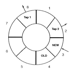
Schematic of a simple digital delay line with taps
In this diagram, we use only 8 samples to keep things
simple, and they are shown as a ring because of the
wrap-around function just explained. Samples are written
in order to the memory locations 1, 2 and in the
diagram, the newest sample is written to memory location
3. That means that memory locations 4 around to 2 are
“old” samples, the oldest being the current value of
location 4 which will be over-written at the next step
of recording. The value of any other of these past
samples can be read as a “
tap”, similar to a
playback head on the tape recorder. The number of taps
determines how many delays can be accessed (in this
diagram, two) and their position can change.
Two issues that arise with delay lines should be
mentioned before we look at various processors and
plug-ins below. The first is how
smoothly the
signal transitions between different delay values. In a
poor implementation there can be
clicks or other
artifacts as the delay values are changed. This is
because there can be discontinuities in the waveform
when samples from different points in time are
encountered during these changes, unless an
interpolation algorithm is used.
The second issue, of particular relevance for phasing,
is how the entire
time range for the delays is
handled. If it is handled linearly, then the critical
range for phasing (less than 10 ms) will be crunched
into a minuscule area of the control interface where it
can’t be properly tuned. At this level of microsound
(less than 50 ms) even 1 ms intervals can make a big
difference in the output. Similarly, large delays may
take a long time to scroll through to find the desired
values. In general, a
logarithmic control
interface is preferable.
In the 1980s when digital memory was
still expensive, a large number of hardware digital
delay units were manufactured, and arguably the Lexicon
models were one of the most prominent. They were quite
expensive and only sold to audio studios, and these now
“classic” modules still command good prices on the used
market.
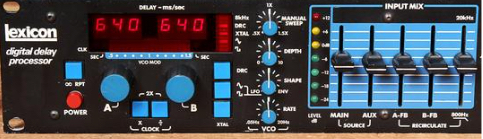
Lexicon
Digital Delay unit
The Lexicon Prime Time II model 95 shown here provided
an excellent control interface for the user. The
version at Simon Fraser University was equipped with
enough memory to allow a maximum 2.56 sec delay to be
realized with two output delays, A & B, that could
be individually set (and doubled with a half sampling
rate). The Input Mix at right allowed a mix of the
original mono signal with the A and B delays treated
as a stereo pair, along with a sensitive feedback
level and a low-pass filter for keeping the
feedback levels from getting too bright. At the low
end of the delay range, millisecond values could be
precisely tuned for phasing.
The most useful part of its operation was the series
of control knobs in the middle which allowed a mix of
various types of modulation of the delays: a
manual sweep, a VCO (voltage-controlled
subaudio oscillator) for modulating with a sine or
square wave with variable frequency and depth, and an
envelope follower for correlating the
delays with the amplitude of the input signal. This
type of correlation was used for the carding wool
phasing examples above.
An “infinite repeat” switch at the left froze
the contents of the memory, similar to a tape loop.
However, the delay taps were still working at
processing the contents of the memory. Therefore, the
doubling of the delay times could lower the pitch by
an octave (similar to playing a loop at half speed),
and changing the VCO and other modulations to create
additional effects. Under the red visual display of
the delays, a “flying beam” gave an effective display
of the instantaneous modulated delays.
Harmonization and other pitch
changes. Even though it’s not about delays, the
delay line itself can be used to change the pitch of
the output, or to modulate it. The general rule is
that when the record and playback rates are equal,
there will be no change in pitch, whether we’re
referring to tape speed or digital sampling rate.
Likewise, when the playback rate is different from
that of the recording, a change in pitch will occur.
For instance, when we step through a delay line one
sample at a time, there’s no pitch change, as long as
the sampling rate hasn't changed. But if we skipped
every other sample (a sample increment of 2)
the sound would rise one octave, and likewise if we
repeated every sample (increment of .5) the sound
would fall an octave. If we stick to integer
increments, such as 1, 2, 3, 4, then those pitches
will all be harmonics, and if those taps are
combined with the original, the effect is called harmonization.
Similarly, when we modulate the delays
regularly, we are actually stepping forwards and
then backwards through the delay line around the
average, and therefore a smooth rise and fall of pitch
will result if the modulator is a sine wave. This kind
of delay
modulation is often called flanging.
It might be thought that there is
no analog equivalent of such pitch changes, but in
fact a specially adapted tape recorder called a tempophone
was designed in Europe to change the pitch of a
recording without altering its duration. The key to
this solution was a rotating set of playback heads,
attached to all sides of the circular mechanism, and
spaced such that one head was always in contact with
the tape.
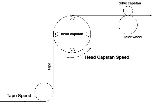 Tempophone
with
rotating heads (click to enlarge)
Tempophone
with
rotating heads (click to enlarge)
Compositional example. Two
voices are reading a text from the Song of Solomon in
Barry Truax’s Song of Songs (1992) which is
processed with a comb filter with various time delays
(i.e. taps), as well as a high-pass filter towards the
end.
|
Text phasing in Song of
Songs |
Click to enlarge
|
Index
D. Echo and feedback at longer
delays. When the time delay for a repetition is
long enough for the auditory system to determine that
it is a separate event, as opposed to being fused with
the original sound, we normally regard the delayed
version as an echo.
Of course, the echo as a separate event depends on the
original sound being relatively short, or at least in
its decay portion before the echo arrives. Otherwise,
with a longer sound, the echo will be masked by
the original and not be heard as a repetition.
The theoretical minimum delay for this kind of
separation is 50 ms, but that can only be
demonstrated in a laboratory situation with very short
clicks heard on headphones. In the case of actual
reverberation, the topic of the next module,
acousticians regard early reflections as those
arriving within the first 80 ms which
reinforce and fuse with the original sound. They also
provide a wider spatial perspective, since the
reflections come from a side angle, but preferably not
too wide. These early reflections are highly desirable
in concert hall acoustics, as discussed in the Sound-Environment
Interaction module.
Besides the duration of the original sound, the other
variable that determines whether a sound is heard as
an echo is its strength (which depends on the
reflectivity of the surface producing the reflection)
and whether the original sound has a sharp attack
and therefore is less likely to mask the echo. If the
delay is longer than 100 ms, and reasonably
strong, it will likely be heard as an echo. As
such it creates a rhythmic relationship with
the original.
Very long delays, on the order of several seconds, can
occur outdoors and have always fascinated listeners.
We talk about “bouncing” a sound off of a distant wall
with a short clap or shout when there is only one
primary surface to produce the reflection. The frequency
response of the surface, as well as reflections
off the intervening ground or water, will colour the
echo, but it always can be recognized as the “same”
sound. Not surprisingly the effect is cited in many
legends and stories where the echo often is regarded
as a manifestation of some “other” being or spirit
that perhaps is answering or mocking us.
Echo
from across a lake
Slap echo under a parabolic bridge
from a handclap
Slap echo in Place Victoria Metro
station, Montréal |
|
Index
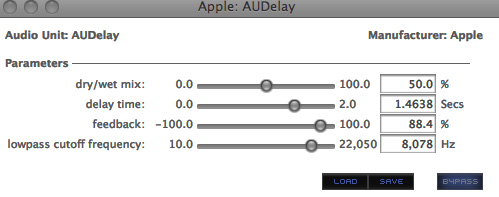
E. Studio demo’s of phasing, echo and
feedback. We will start with a very simple but
typical delay processor with just the four most basic
parameters: (1) the traditional dry/wet mix
expressed as a percentage of how much processed (i.e.
wet) sound is mixed with the original (i.e. the dry
sound); (2) the delay time in seconds (max. 2)
which uses decimal places but will be very difficult to
tune in the low phasing region as the steps are too
large; (3) feedback level in percentage up to
100% with a negative version that inverts the phase of
the feedback and (4) a low-pass cutoff frequency
to minimize the brightness level of the feedback. There
are no separate controls for each stereo channel.
Next we will consider the standard plug-ins used in the
Audition editor for processing. The carding sound used
earlier in the phasing demo’s will be used again as a
source for comparison. The two examples are of phasing
and what the software calls flanging.
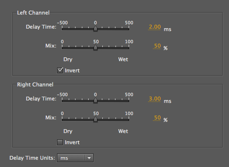
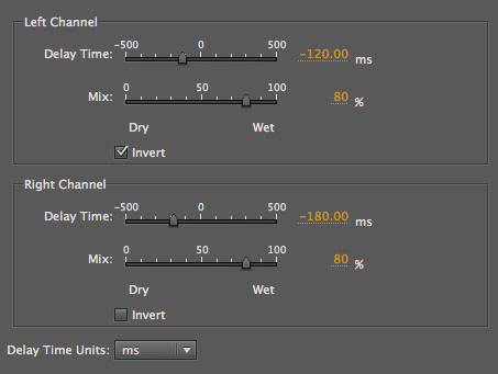
In the Delay plug-in, which we will use to
produce phasing, delay times in milliseconds
allow a very precise value to be typed in, with separate
values for the left and right channels, in this case 2
and 3 ms. Given that it is difficult to use the slider
in the middle for such precise values, it is easier to
type in the desired number (or drag the parameter value
which increments by .1 ms). The wet/dry mix (i.e.
original + processed) should be set to 50% for each
since the intent is probably to have the strongest
effect.
A nice option here is to invert the signal on
one or both channels. This means that the cancelled
frequencies are shifted. Given that Audition allows the
left and right channels to be soloed during this process
(which works best with the loop playback on), one can
hear the differences easily, even though they fuse in
the stereo version (as you can tell by listening to one
channel, then the other).
Carding with stereo phasing
Source: WSP Can 33 take 1& 2
|
|
Carding with Flange
|
|
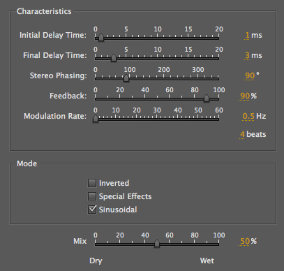
In the Flange example, it’s
all about modulation. The top two controls
allow you to choose the minimum and maximum (labelled
initial and final) delays in the sinusoidal
modulation, plus the all-important rate at the
bottom. In this case, we chose a very slow subaudio
rate (0.5 Hz which means the cycle is 2 sec), so the
effect would be subtle, but this can still be heard as
a slow upward and downward pitch proceeding
independent of the sound. Feedback was set to 90% to
add a somewhat harmonic pitch to the result.
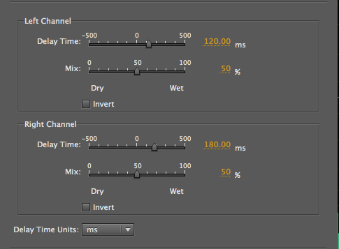
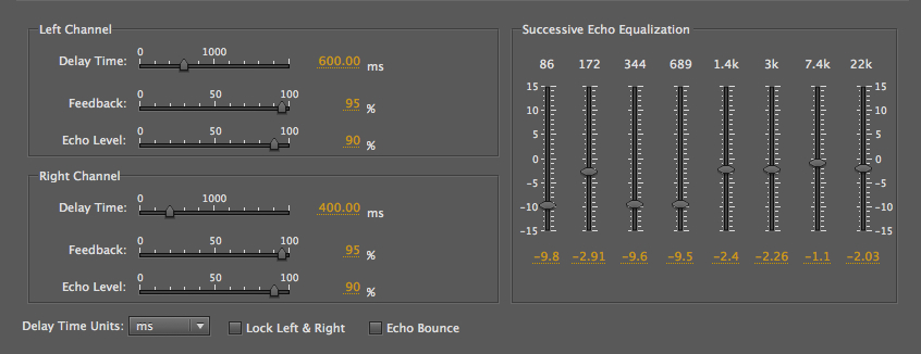
Next we use Audition’s Delay & Echo plug-ins with
longer delays applied to create rhythmic
enhancements of this short hammering on wood
recording, which you can download here (control click
or right click). However the delays can either follow
the original (plus values) or precede it
(negative values), a choice that wouldn’t be available
in the analog domain. By adjusting the dry/wet
percentages, an interesting psychoacoustic effect
occurs. When the mix is 50/50, we hear the echo as rhythmic
enhancement. But when it is 80% wet and precedes the
original, then the latter is heard as a spatial
echo. Note that a similar effect could be
specified with the echo following the original at 20%,
but with a slightly different rhythm.
Hammering with L/R rhythmic
additions of 120 and 180 ms delays
|
|
The echoes now precede each hit
which is heard as a spatial echo
|
|
The Echo plug-in is actually a
misnomer as the delays are only heard when the
feedback level is brought up, so multiple days are
always heard. This becomes a feedback circuit
which raises a difficult issue with how we do this
process in editors – it can be heard dynamically with
the build up of feedback levels, but when applied
permanently, there is no additional duration
added, and so we are getting only the first pass of
the buildup. This problem will be addressed
differently below.
Hammering rhythm with feedback
|
|
In fact, in order to avoid the feedback being abruptly
curtailed, we had to add several seconds of
silence, as in this example, if we want to hear the
feedback continue. By taking the process out of real
time (which was the only option in the analog domain),
the process is frozen into a single pass of the
circuit. On the other hand, in this plug-in, there is
a useful EQ at the right where the spectrum can be
adjusted, even if it is done just once.
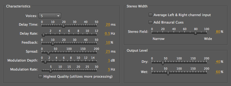
Finally we listen to the process of
digital Chorusing, which as discussed above,
is not the same as the acoustic choral
effect where multiple voices blend
together with small de-tunings and staggered entry
delays. This is Audition’s version of a 5-voice
chorusing with a bass voice. As you can see from the
parameters, modulation is being used to create the
illusion of small pitch shifts, but in fact, one can
still hear the modulation going on. But, it’s still a
very enriched sound.
5-voice chorusing with a bass
voice
(Derrick
Christian)
|
|
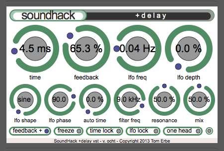
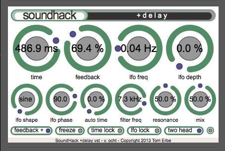
A different, more graphic approach
to many of the same variables can be found with
SoundHack’s Delay Line (part of the free
download called the Delay Trio). The lefthand
screenshot shows a typical phasing setting. The slider
knob is intelligently calibrated in a logarithmic
manner, so that very small time delays needed
for phasing are in 0.2 ms steps, whereas for long
delays (max 5 sec) the steps are much larger. As a
result, the delays are very easy to adjust. The
righthand screenshot shows a typical rhythmic delay
setting (just under .5 sec), with about 70% feedback.
This is one of the few apps where a feedback control
is allowed to exceed 100%, indicating that
this module is designed for live performance, where
the level can be brought back down again quickly.
Most of the other sliders (shown as knobs)
control the rate, depth and phase of the delay
modulation, along with a slider at the lower left
which switches from sine to triangle, square, up and
down ramps, and random. Resonance can also be added to
the low-pass filter as a percentage. The switches at the
bottom can change the feedback from + to -,
which is useful in phasing. Possibly influenced by the
Lexicon “infinite repeat” button shown above, the memory
can be frozen as a loop. The last switch at the
bottom right brings in two delay taps which are
cross-faded and used to smooth the steps in a ramp.
Recording dynamic processes that
use feedback. As discussed in the previous module,
recording interactive changes in any of these
modules is not part of the plug-in paradigm.
Interactivity is assumed to only be relevant while you
are testing and adjusting the settings, then you “apply”
them, and the result is fixed. We also discussed in that
previous module some solutions that could be applied,
such as recording the output to another program, but in
a laptop situation, for instance, that is not possible.
Instead, we showed a simple DAW design for automating
parameters in a session and recording changes in
individual parameter settings the same way one records
mixing levels, i.e. by latching them. In this
module we have commented on a particularly difficult
process to integrate into digital software, namely an
active feedback circuit.
In the analog circuits we have shown, it was taken for
granted that the result, of any length, could be stored
on tape. However, the plug-in paradigm allows the
process to be stored only in the same length as
the original file, and therefore it arbitrarily cuts off
the sound of the feedback tail. The only easy solution
is to add several seconds of silence if you want
to capture that slow decay.
On the other hand, if we were to program to feedback
level in a DAW session, such that it fell back to zero
at the end, it wouldn’t take long for the feedback sound
to disappear. Of course it could also be raised and
lowered during the sound itself by the same method. Here
is a simple example that illustrates a direction that
could be followed (click to enlarge)
Feedback mix with automated levels
|
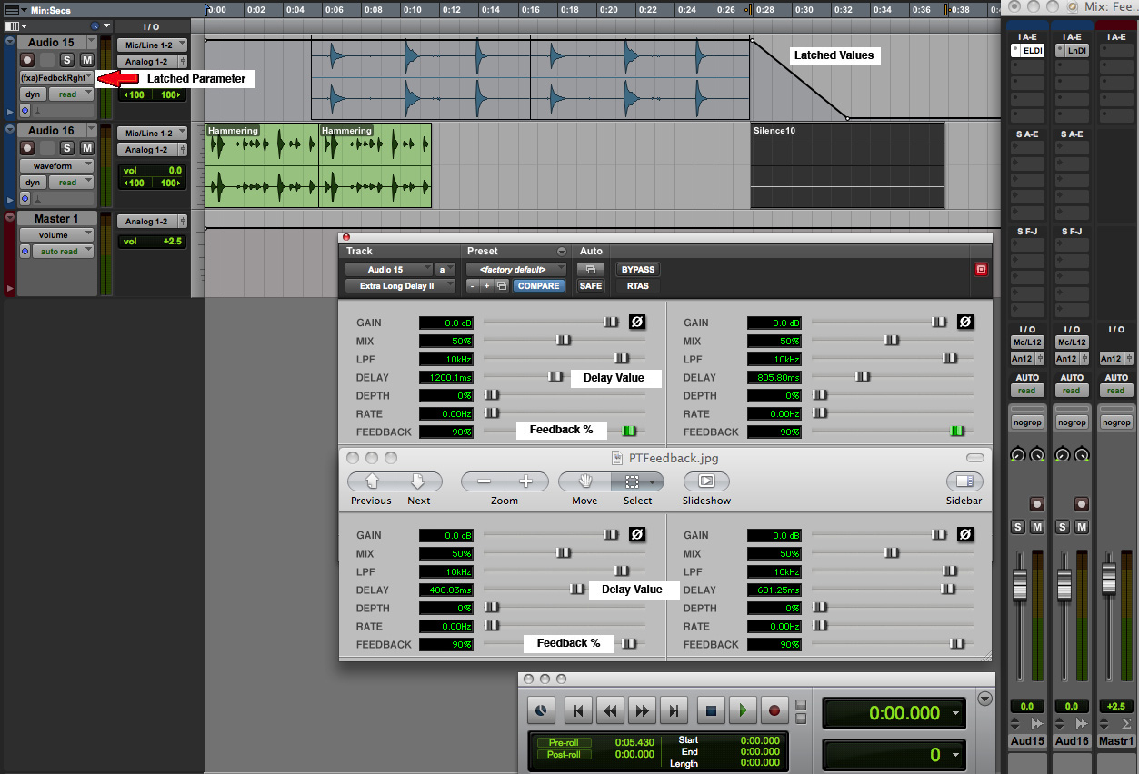
Click to enlarge |
We
start with the hammering (green track) used above with
two short stereo delays (400 and 600 ms) and 90%
feedback. We then bring in another rhythmic sound, the
PVC pipe (blue track) with delays of 800 and 1200 ms,
and that allows the hammering feedback to continue
without adding any silence. Then at the end of the PVC
track, we add 10 seconds of silence to allow its
feedback to continue. However, in general it’s hard to
calculate how long that might last. So, the most elegant
solution is to automate the feedback level, both
left and right versions, and ramp them down at the end.
This feedback level control is shown on the top track.
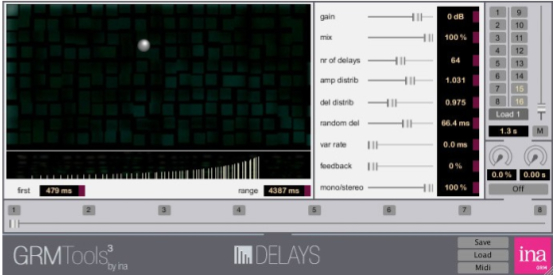
Finally we will make a brief reference
to two very rich processes offered in GRM Tools,
namely Delays and Comb. With the former,
you are offered an array of up to 128 delay lines (!)
with a clever means of distributing them, weighted
towards the top in terms of spacing, as shown, or
towards the bottom, or even throughout; amplitude
distributions increasing as shown, or decreasing. Some
degree of randomness can be added, as well as feedback
levels. Unless you limit yourself to a subset of these
parameters, the effect will be very strong – and will
tend to dominate everything else in a mix.
|
|
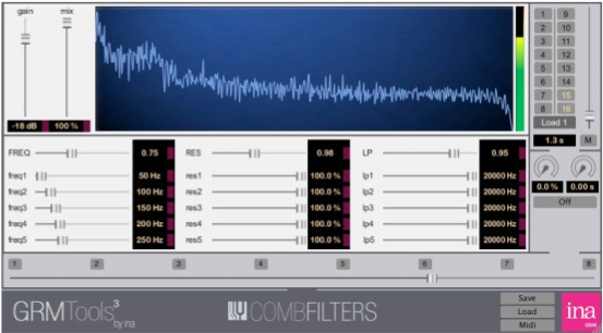
The comb filter is also quite grand, offering a
bank of 5 comb filters, all individually tunable, with
varying degrees of resonance (i.e. feedback) to add a
rich harmonic spectrum, low-pass filters on each comb to
manage the brightness, and a global frequency shifter
for upward and downward transposition, as well as global
controls for the resonance and low-pass filtering.
Again, very impressive, but must be handled with care!
Personal Studio
Experiments. If you have been following
the personal studio experiments suggested in the
previous two EA modules, you will find a lot of scope
for extensions of those materials in this module.
First you need to examine the available plug-ins you
have for the time domain and try to identify the key
control elements as discussed here. Pay particular
attention to the lowest delay range to see if it is
amenable to very small steps as shown for phasing.
If
you are experimenting with rhythmic variants created
with echoes, you’ll need some time to find the correct
time values that will work with your rhythmic sounds
and/or loops. If you start to experiment with
feedback, you’ll have to find the means to deal with
its dynamic behaviour, both in terms of the effects
produced, and the problem of recording them. If you’ve
already created some DAW circuits especially designed
for processing, as suggested in previous modules, you
may want to do the same for feedback processes as
suggested here.
In
terms of composition, everything is open-ended of
course, but it might be wise to have fully explored
the timbral domain changes (including pitch), and now
the temporal domain processes, before you start
constructing a mixing session. The two domains,
frequency and time, work quite differently and produce
different kinds of results, so in terms of exploring
your material, both areas should be thoroughly tried
out.
Index
Q. Try this review quiz to
test your comprehension of the above material,
and perhaps to clarify some distinctions you may
have missed.
home