STAT 330 Lecture 30

Reading for Today's Lecture: 12.1, 12.2,12.3

Goals of Today's Lecture:

• Learn confidence interval and hypothesis testing procedures for the slope in a simple linear regression.
• Learn to make and examine residual plots in simple linear regression.

Today's notes

Simple Linear Regression Model:

We assume for each observation a model equation of the form

where

• Y is the response or dependent variable.
• is the (fixed) value of a covariate.
• is the slope and the intercept of a straight line.
• the are independent mean 0 errors with constant variance .

Distribution theory for estimates:

1. The least squares estimates and minimize

   

   and are given by

   

   and

   

   where

   

2. The standard deviation, , of the errors is estimated by

   

3. Other formulas, useful for computing means and variances are:

   

   and

   

4. and are unbiased:

   

   and

   

5. 
6. is an unbiased estimate of

   If we also assume that the errors are then

7. the least squares estimates are also the maximum likelihood estimates.
8. has a normal distribution with mean and variance NOTE: in samples where the largest is small compared to (most large samples) this normality is approximately true even if the errors do NOT have a normal distribution.
9. are independent of s.
10. has a distribution on n-2 degrees of freedom.
11. The pivot

    

    has a t distribution on n-2 degrees of freedom.

We can use this distribution theory to test hypotheses and give confidence intervals:

Confidence Intervals

The inequality can be solved as usual to get the interval

This confidence interval, which is exact for normally distributed errors can also be used in large samples for non-normal errors.

Hypothesis Tests

We can test by computing

and getting P values from t tables. Again this test can be used in large samples even if the errors are not normal. The most common value for is 0. In this case

and

is the F statistic from the ANOVA table.

Residual Plots

After fitting the model you should examine residual plots. The fitted residuals are defined by

You should plot:

• Residual against x. Look for
  • Non constant variance. Does the vertical spread change as x changes?
  • A trend in the residuals. If the plot of residuals is curved then there is evidence that the straight line regression function is inappropriate.
  • Y outliers. If any of the residuals are much larger than the others then there is evidence that the model does not fit for that data point.
  • x outliers. If any of the data points has an x value far away from the others then that observation is called influential; it may have a big impact on the estimated slope and intercept.

• Residual against fitted value, . Look for the same features as in the previous plot. Note: this plot is more useful in multiple regression. For simple linear regression this plot is the same as the plot of against x except for the label on the x axis.
• a Q-Q plot of the residuals (also called a normal probability plot) to check to see if the residuals seem to have a normal distribution.
• Residual versus the order in which the data were collected (if available). Look for trends with time; our model predicts no such trends.

Example: see text chapter 12 question 9.

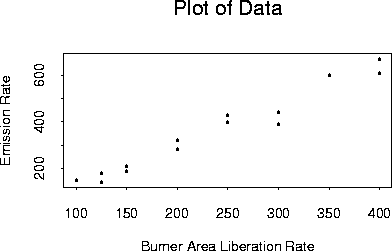
An experiment was conducted to relate a variable Y, the production of nitrous oxides to a variable x, the "Burner Area Liberation Rate" (a measure of energy produced per square foot of area of some burner in a power plant). The data are

x 100 125 125 150 150 200 200

y 150 140 180 210 190 320 280

x 250 250 300 300 350 400 400

y 400 430 440 390 600 610 670

Here is a plot of the data:

I used SAS to fit the regression model. In particular I used proc glm (glm stands for general linear model). Here is the SAS code:

  options pagesize=60 linesize=80;
  data nox;
  infile 'ch12q9.dat';
  input area emission ;
  proc glm  data=nox;
   model emission = area;
   output out=noxfit p=yhat r=resid ;
  proc univariate data=noxfit plot normal;
   var resid;
  proc plot;
   plot resid*area;
   plot resid*yhat;
  run;

The line labelled model says that I am interested in the effects of area (my shorthand name for ``Burner Area Liberation Rate'') on emissions.

The output from proc glm is

                        The SAS System                                1
                                        10:00 Monday, November 20, 1995

               General Linear Models Procedure

           Number of observations in data set = 14

                        The SAS System                                2
                                        10:00 Monday, November 20, 1995

               General Linear Models Procedure

Dependent Variable: EMISSION
                         Sum of            Mean
Source          DF      Squares          Square     F Value     Pr > F

Model            1   398030.26093    398030.26093    294.74     0.0001

Error           12    16205.45335      1350.45445

Corrected Total 13   414235.71429

      R-Square             C.V.        Root MSE        EMISSION Mean

      0.960879         10.26905       36.748530            357.85714


Source      DF        Type I SS     Mean Square   F Value     Pr > F

AREA         1     398030.26093    398030.26093    294.74     0.0001

Source      DF      Type III SS     Mean Square   F Value     Pr > F

AREA         1     398030.26093    398030.26093    294.74     0.0001


                                  T for H0:    Pr > |T|   Std Error of
Parameter            Estimate    Parameter=0                Estimate

INTERCEPT        -45.55190539          -1.79     0.0989    25.46779420
AREA               1.71143233          17.17     0.0001     0.09968772

The conclusions are that AREA has a very significant and strong effect on emissions, that the intercept of the linear regression might be 0 and that the estimated slope is

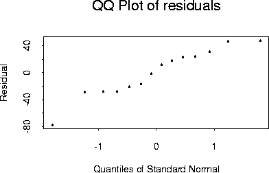
The diagnostic plots show one possible Y outlier at x=300

            Plot of RESID*AREA.  Legend: A = 1 obs, B = 2 obs, etc.
RESID |
      |
   60 +
      |
      |
      |
      |                                    A                       A
      |
   40 +
      |
      |
      |                                                                        A
      |
      |A                       A
   20 +
      |                                    A
      |
      |      A
      |
      |
    0 +            A
      |
      |
      |
      |
      |                        A
  -20 +            A
      |
      |                                                A
      |      A                                                                 A
      |
      |
  -40 +
      |
      |
      |
      |
      |
  -60 +
      |
      |
      |
      |
      |                                                A
  -80 +
      |
      -+-----+-----+-----+-----+-----+-----+-----+-----+-----+-----+-----+-----+
      100   125   150   175   200   225   250   275   300   325   350   375  400
                                         AREA

Here is a Q-Q plot of the residuals

Prediction Intervals

University admissions officers would like to guess a student's GPA at the end of first year on the basis of her/his high school record. In the simplest case that high school record might be summarized by x, the high school GPA. The mathematical version of this problem is that there is a data set of pairs and a new individual x for which we desire to guess the corresponding Y. A related, but different problem is to guess the average first year GPA for a large group of students whose high school GPA is x.

We will use the following notation.

• is a prediction of the Y value of a new individual.
• is the expected value of Y corresponding to a given x. For simple linear regression

  

If we have fitted a simple linear regression model to our data set, obtaining estimated slope and intercept then we predict both the individual and the average of the group using the regression line:

Next lecture we will develop the theory to get an estimate of the likely size of the prediction error , a prediction interval for Y (of the form ) and a standard error and confidence interval for .