No Title

STAT 350: Lecture 32

Example: transformation vs glm

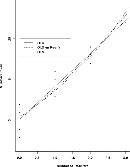
At each of 5 doses of some drug 40 animals were tested and the number dying were recorded. The log doses are -3.204, -2.903, -2.602, -2.301, and -2.000 and the numbers surviving are 7, 18, 32, 35, 38. A plot of the data is

After the arcsine transform we have

A more standard transformation for this problem is the logit or logistic

$\begin{displaymath}Y_i^* = \log[Y_i/(n_i-Y_i)] \end{displaymath}$

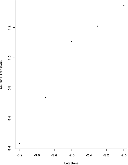
Here is the data analyzed by least squares after the logistic transformation

THE DATA FILE

Dose   Dead  Tested
-3.204    7     40
-2.903   18     40
-2.602   32     40
-2.301   35     40
-2.000   38     40

I used SPlus to analyze the data; here is a file full of commands I used.

dead <- read.table("data", header = T)
attach(dead)
postscript("logist.ps",onefile=F,horizontal=F)
plot(Dose, Dead/Tested,xlab="Log Dose",
     ylab="Proportion Dying")
dev.off()
postscript("arc_logist.ps",onefile=F,horizontal=F)
plot(Dose, Dead/Tested,xlab="Log Dose",
     ylab="Arc Sine Transform")
dev.off()
postscript("logit_logist.ps",onefile=F,horizontal=F)
plot(Dose, log(Dead/(Tested-Dead)),xlab="Log Dose",
     ylab="Logit Transform")
dev.off()
linfit <- lm( log(Dead/(Tested-Dead)) ~ Dose, data=dead)
summary(linfit)
glmfit <- glm( cbind(Dead,Tested-Dead) ~ Dose, 
     data=dead, family=binomial)
summary(glmfit)
postscript("logist_plus_curve.ps",onefile=F,horizontal=F)
plot(Dose, Dead/Tested,xlab="Log Dose",
     ylab="Proportion Dying")
d <- seq(-3.3,-1.9,length=200)
etalin <- coef(linfit)[1] + d*coef(linfit)[2]
p  <- exp(etalin)/(1+exp(etalin))
lines(d,p)
etaglm <- coef(glmfit)[1] + d*coef(glmfit)[2]
p  <- exp(etaglm)/(1+exp(etaglm))
lines(d,p,lty=2)
dev.off()

The output consists of 4 postscript files which have graphs in them and the following printout:

S-PLUS : Copyright (c) 1988, 1996 MathSoft, Inc.
S : Copyright AT&T.
Version 3.4 Release 1 for Sun SPARC, SunOS 5.3 : 1996 
Working data will be in .Data 
> dead <- read.table("data", header = T)
#
#    Read in the data.  Columns are named by the words 
#    read off line 1 because of the header=T bit.
#
> attach(dead)
#
#    Makes the variable which are columns of dead
#    accessible to the plotting rooutines
#
> postscript("logist.ps",onefile=F,horizontal=F)
#
#    Declares that the next graph should be put
#    in a postscript file called logist.ps.  The 
#    file should be encapsulated postscript and in 
#    portrait orientation.
#
> plot(Dose, Dead/Tested,xlab="Log Dose",
     ylab="Proportion Dying")
#
#    Plot Proportion dying on the y axis against 
#    Dose and label the axes
#
> dev.off()
#
#    Finish up the postscript file
#
Starting to make postscript file.
Finished postscript file, 
     executing command "lpr -h logist.ps &".
 null device 
           1
> postscript("arc_logist.ps",onefile=F,horizontal=F)
> plot(Dose, asin(sqrt(Dead/Tested)),xlab="Log Dose",
     ylab="Arc Sine Transform")
> dev.off()
Starting to make postscript file.
Finished postscript file, 
     executing command "lpr -h arc_logist.ps &".
 null device 
           1
> postscript("logit_logist.ps",onefile=F,horizontal=F)
> plot(Dose, log(Dead/(Tested-Dead)),xlab="Log Dose",
     ylab="Logit Transform")
> dev.off()
Starting to make postscript file.
Finished postscript file, 
     executing command "lpr -h logit_logist.ps &".
 null device 
           1
> linfit <- lm( log(Dead/(Tested-Dead)) ~ Dose, data=dead)
#
#   Regress log(Y/(n-Y)) on Dose
#
> summary(linfit)
#
#   Print out a summary of the regression results.
#
Call: lm(formula = log(Dead/(Tested - Dead)) ~ Dose, 
     data = dead)
Residuals:
       1       2      3        4      5 
 -0.2283 0.00792 0.4812 -0.07283 -0.188

Coefficients:
              Value Std. Error t value Pr(>|t|) 
(Intercept) 10.5322  0.9109    11.5626  0.0014 
       Dose  3.6999  0.3455    10.7095  0.0017 

Residual standard error: 0.3288 on 3 degrees of freedom
Multiple R-Squared: 0.9745 
F-statistic: 114.7 on 1 and 3 degrees of freedom, 
     the p-value is 0.001741 

Correlation of Coefficients:
     (Intercept) 
Dose 0.9869     
> glmfit <- glm( cbind(Dead,Tested-Dead) ~ Dose, 
     data=dead, family=binomial)
# 
#   This fits the model that log(E(Y)/(n-E(Y)) is 
#   a linear function of Dose
#
> summary(glmfit)

Call: glm(formula = cbind(Dead, Tested - Dead)~Dose, 
     family = binomial, data = dead)
Deviance Residuals:
          1           2        3         4          5 
 -0.4319303 -0.03563685 1.026423 -0.476305 -0.5453582

Coefficients:
                Value Std. Error  t value 
(Intercept) 11.238232  1.5651480 7.180300
       Dose  3.936472  0.5604985 7.023162

(Dispersion Parameter for Binomial family 
     taken to be 1 )

    Null Deviance: 80.77441 on 4 degrees of freedom

Residual Deviance: 1.76566 on 3 degrees of freedom

Number of Fisher Scoring Iterations: 3 

Correlation of Coefficients:
     (Intercept) 
Dose 0.9929832  
> 
> postscript("logist_plus_curve.ps",onefile=F,
     horizontal=F)
> plot(Dose, Dead/Tested,xlab="Log Dose",
     ylab="Proportion Dying")
> d <- seq(-3.3,-1.9,length=200)
> etalin <- coef(linfit)[1] + d*coef(linfit)[2]
> p  <- exp(etalin)/(1+exp(etalin))
#
#    For each dose in d, which is a list of 200 numbers 
#    running from -3.3 to -1.9, compute the fitted 
#    probability according to the logit model: 
#    if log(x/(1-x))=p   then p=exp(x)/(1+exp(x))
#
> lines(d,p)
#
#   Plot the fitted curve for the least squares 
#   method on the graph of the data
#
> etaglm <- coef(glmfit)[1] + d*coef(glmfit)[2]
> p  <- exp(etaglm)/(1+exp(etaglm))
#
#    Do the same for the generalized model fit
#
> lines(d,p,lty=2)
#
#   Plot the fitted curve for the glm method on the 
#   graph of the data.  Use a dashed (lty=2) line.
#
> dev.off()
Starting to make postscript file.
Finished postscript file, 
    executing command "lpr -h logist_plus_curve.ps &".
 null device 
           1
> q() # end-of-file

The slopes of the two fits differ by about one half of one standard error.
The function glm fits a generalized linear model, using maximum likelihood methods for a binomial model for the number of dead animals at each dose.
The standard errors produced by glm are more appropriate and larger. The linear model fit assumes homoscedasticity which is definitely wrong for binomial data.
The two fitted curves are plotted along with the data in the last set of lines.

Poisson Regression: Count Data

In the table below the first row is the number of times a carton of glass objects was transferred from one aircraft to another during shipping. The second row is the number of broken objects.

i:	1	2	3	4	5	6	7	8	9	10
X_i	1	0	2	0	3	1	0	1	2	0
Y_i	16	9	17	12	22	13	8	15	19	11

A reasonable model is that Y_i has a Poisson distribution with mean $\mu_i$ which depends in some way on X_i. We fit 3 models:

1.

The ordinary linear regression model

$\begin{displaymath}Y_i=\beta_0+\beta_1 X_i + \epsilon_i \end{displaymath}$

for which the relevant plot is

2.

The transformed regression model

$\begin{displaymath}\sqrt{Y_i} = \beta_0 + \beta_1X_i + \epsilon_i \end{displaymath}$

for which the relevant plot is

3.

The Poisson regression model in which Y_i has a Poisson( $\mu_i$ ) distribution and

$\begin{displaymath}\log\mu_i = \beta_0+\beta_1 X_i\end{displaymath}$

or equivalently

$\begin{displaymath}\mu_i = \exp(\beta_0+\beta_1 X_i) \end{displaymath}$

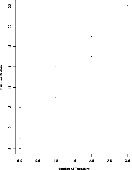
The following SPlus code fits these models

dat <- read.table("data", header = T)
attach(dat)
postscript("xyplot.ps",onefile=F,horizontal=F)
plot(Transfers,Broken,
     xlab="Number of Transfers",
     ylab="Number Broken")
dev.off()
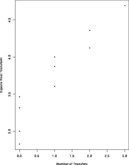
postscript("xrootyplot.ps",onefile=F,horizontal=F)
plot(Transfers, sqrt(Broken),
     xlab="Number of Transfers",
     ylab="Square Root Transform")
dev.off()
#
#   Regress Number Broken on Number of Transfers
#
linfit <- lm( Broken ~ Transfers, data=dat)
summary(linfit)
diag(linfit)
#
#   Regress Square Root of Number Broken 
#     on Number of Transfers
#
rootlinfit <- lm( sqrt(Broken) ~ Transfers, data=dat)
summary(rootlinfit)
diag(rootlinfit)
# 
#   The following fits log(E(Y)) is a linear function
#   of Dose and variance is equal to the mean
#
glmfit <- glm( Broken ~ Transfers, data=dat, 
     family=Poisson)
summary(glmfit)
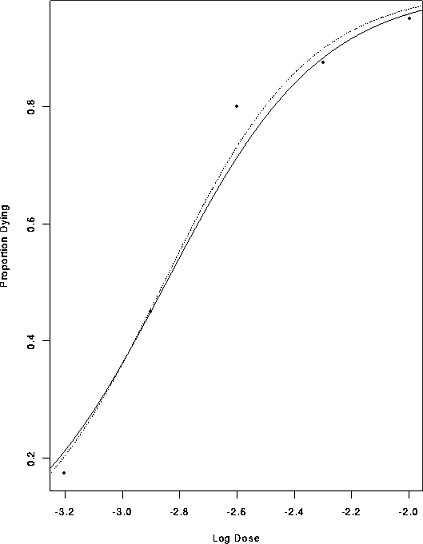
postscript("points_plus_curve.ps",onefile=F,horizontal=F)
plot(Transfers,Broken,xlab="Number of Transfers",
     ylab="Number Broken")
d <- seq(0,4,length=200)
etalin <- coef(linfit)[1] + d*coef(linfit)[2]
lines(d,etalin)
etarootlin <- coef(rootlinfit)[1] + d*coef(rootlinfit)[2]
lines(d,etarootlin^2,lty=2)
etaglm <- coef(glmfit)[1] + d*coef(glmfit)[2]
p  <- exp(etaglm)
lines(d,p,lty=3)
legend(0,20,lty=1:3,legend=c("OLS","OLS on Root Y","GLM"))
dev.off()

EDITED OUTPUT (Complete output.)

> summary(linfit)

Call: lm(formula = Broken ~ Transfers, data = dat)
Residuals:
  Min   1Q Median  3Q Max 
 -2.2 -1.2    0.3 0.8 1.8

Coefficients:
              Value Std. Error t value Pr(>|t|) 
(Intercept) 10.2000  0.6633    15.3771  0.0000 
  Transfers  4.0000  0.4690     8.5280  0.0000 

Residual standard error: 1.483 on 8 degrees of freedom
Multiple R-Squared: 0.9009 
F-statistic: 72.73 on 1 and 8 degrees of freedom, 
     the p-value is 2.749e-05 

Correlation of Coefficients:
          (Intercept) 
Transfers -0.7071    

> summary(rootlinfit)

Call: lm(formula = sqrt(Broken) ~ Transfers, data = dat)
Residuals:
     Min      1Q  Median     3Q   Max 
 -0.3722 -0.1263 0.01059 0.1392 0.274

Coefficients:
              Value Std. Error t value Pr(>|t|) 
(Intercept)  3.2006  0.1010    31.6789  0.0000 
  Transfers  0.5254  0.0714     7.3538  0.0001 

Residual standard error: 0.2259 on 8 degrees of freedom
Multiple R-Squared: 0.8711 
F-statistic: 54.08 on 1 and 8 degrees of freedom, 
     the p-value is 7.965e-05 

Correlation of Coefficients:
          (Intercept) 
Transfers -0.7071    

> summary(glmfit)

Call: glm(formula = Broken ~ Transfers, 
     family = poisson, data = dat)
Deviance Residuals:
        Min         1Q      Median        3Q       Max 
 -0.8105292 -0.2389281 -0.02029464 0.3299091 0.6074179

Coefficients:
                Value Std. Error   t value 
(Intercept) 2.3529495  0.1317376 17.860883
  Transfers 0.2638422  0.0792345  3.329891

(Dispersion Parameter for Poisson family taken to be 1 )

    Null Deviance: 12.56868 on 9 degrees of freedom

Residual Deviance: 1.813176 on 8 degrees of freedom

Number of Fisher Scoring Iterations: 3 

Correlation of Coefficients:
          (Intercept) 
Transfers -0.770864

The fits together

$next$ $up$ $previous$

Richard Lockhart
1999-03-23