is a density.
- (a)
- Let
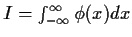 .
Show that
.
Show that

HINT: What is in terms of I.
Solution
We have
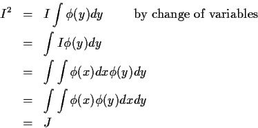
- (b)
- Now if

do the double integral J in polar co-ordinates ( ,
,
 )
to show J=1.
)
to show J=1.
Solution
When you do an integral in polar co-ordinates you have to: replace each x in the integrand with
 and each ywith
 ,
replace dxdy with
,
replace dxdy with
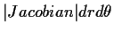 ,
and find the set of
,
and find the set of  values which correspond to the set
of x,y values over which we are integrating. The Jacobian is the
absolute value of the determinant filled up with derivatives of (x,y)with respect to r and
values which correspond to the set
of x,y values over which we are integrating. The Jacobian is the
absolute value of the determinant filled up with derivatives of (x,y)with respect to r and  .
This 2 by 2 matrix has determinant
r. The value of r, being a distance from the origin is in the
range 0 to
.
This 2 by 2 matrix has determinant
r. The value of r, being a distance from the origin is in the
range 0 to  while the angle in the plane is measured over
any interval of length
while the angle in the plane is measured over
any interval of length  such as
  .
This makes
.
This makes

The
integral gives
leaving

- (c)
- Deduce that
 is a density.
Solution
All you have to do is prove that
 and
and
 .
But
is clearly positive. Thus I>0 and since I2=J=1we have I=1.
.
But
is clearly positive. Thus I>0 and since I2=J=1we have I=1.
 random
variables, so that
random
variables, so that
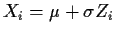 with
Z1,Z2,Z3 independent
standard normals.
with
Z1,Z2,Z3 independent
standard normals.
- (a)
- If
XT = (X1,X2,X3) and
ZT=(Z1,Z2,Z3) express X in the
form AZ+b for a suitable matrix A and vector b.
Solution
We have
 and
and
![$b^T = [\mu,\mu,\mu]$](img25.gif) .
.
- (b)
- Show that X is
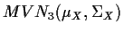 and identify
  and
and  .
.
Solution
The definition of MVN is that X be of the form AZ+b and then
 and
and
 .
So
.
So
![$\mu_x^T= [\mu,\mu,\mu]$](img31.gif) and
and
 .
.
- (c)
- Let
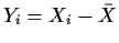 for i=1,2,3 and
 .
Show
that
.
Show
that
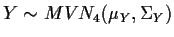 and find
  and
and  .
.
Solution
Let B be the matrix
![\begin{displaymath}B = \left[\begin{array}{rrr}
2/3 & -1/3 & -1/3 \\
-1/3 & 2/3...
...
-1/3 & -1/3 & 2/3 \\
1/3 & 1/3 & 1/3
\end{array}\right]
\, .
\end{displaymath}](img38.gif)
Then Y=BX so Y is
 .
.
Arithmetically we find
![\begin{displaymath}\mu_Y^T = (B\mu_x)^T = [0,0,0,\mu]
\end{displaymath}](img40.gif)
and
![\begin{displaymath}\Sigma_Y = \sigma^2\left[\begin{array}{rrrr}
2/3 & -1/3 & -1/...
... & -1/3 & 2/3 & 0 \\
0 & 0 & 0 & 1/3
\end{array}\right]\, .
\end{displaymath}](img41.gif)
![$X=[{\bf 1}\vert X_1\vert X_2]$](img42.gif) where Xi has picolumns.
where Xi has picolumns.
- (a)
- Write XTX as a partitioned (3 rows, 3 columns) matrix.
Solution
![\begin{displaymath}X^TX = \left [ \begin{array}{ccc}
n & 1^T X_1 & 1^t X_2 \\
X...
..._2 \\
X_2^T 1 & X_2^T X_1 & X_2^TX_2
\end{array}\right] \, .
\end{displaymath}](img43.gif)
- (b)
- A matrix
![\begin{displaymath}A = \left[\begin{array}{ccc}
A_1 & 0 & 0 \\
0 & A_2 & 0 \\
0 & 0 & A_3
\end{array}\right]
\end{displaymath}](img44.gif)
is called block diagonal. Show that A-1 exists if and only if each Ai-1 exists and that then A-1is block diagonal.Solution
Check by multiplying that
![\begin{displaymath}\left[\begin{array}{ccc}
A_1 & 0 & 0 \\
0 & A_2 & 0 \\
0 & ...
...
I & 0 & 0 \\
0 & I & 0 \\
0 & 0 & I
\end{array}\right] \, .
\end{displaymath}](img45.gif)
This shows that if each Ai is invertible then so is A. I notice in marking that many of you assumed that each Ai was a scalar so that would make sense. That would
make A diagonal, not block diagonal and would be useless for
the next part of this question.
To do the converse suppose that B is A-1 and partition Binto a
would make sense. That would
make A diagonal, not block diagonal and would be useless for
the next part of this question.
To do the converse suppose that B is A-1 and partition Binto a  array with entries Bij. Multiply AB and
set this equal to the identity. You get 9 equations like
A1 B1,1 =I and
A1 B1,2 = 0. The first such
equation shows that A1 must be invertible and that B1,1 must
be the inverse of A1. The second equation then shows (because
we now know that A1 is invertible that B1,2=0. Continue like
this.
array with entries Bij. Multiply AB and
set this equal to the identity. You get 9 equations like
A1 B1,1 =I and
A1 B1,2 = 0. The first such
equation shows that A1 must be invertible and that B1,1 must
be the inverse of A1. The second equation then shows (because
we now know that A1 is invertible that B1,2=0. Continue like
this.
- (c)
- Suppose that
 for i=1,2 and
X1TX2=0.
Show that XTX is block diagonal and give a formula for
(XTX)-1.
for i=1,2 and
X1TX2=0.
Show that XTX is block diagonal and give a formula for
(XTX)-1.
Solutions
The conditions show that all the off-diagonal blocks are 0, remembering that (AB)T = BTAT. Thus
![\begin{displaymath}(X^TX)^{-1} = \left[\begin{array}{ccc}
1/n &0 & 0 \\
0 & (X_1^TX_1)^{-1} & 0 \\
0 & 0 & (X_2^TX_2)^{-1}
\end{array}\right]
\end{displaymath}](img49.gif)
Many students appeared not to realize that because
 is a vector all of whose entries equal the number 1.
- (d)
- Suppose
![$\beta^T = [ \beta_0\vert \beta_1^T\vert\beta_2^T]$](img52.gif) is partitioned
to conform with the partitioning of X (that is
is partitioned
to conform with the partitioning of X (that is  is a scalar
and
is a scalar
and  is a column vector of length pi for i=1,2.
Let
is a column vector of length pi for i=1,2.
Let
 be obtained by fitting

by least square, be obtained by fitting
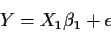
and similarly for .
Let
.
Let  be the usual
least squares estimate for
be the usual
least squares estimate for
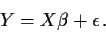
Show that![$\hat\beta^T = [ \tilde\beta_0\vert \tilde\beta_1^T\vert\tilde\beta_2^T]$](img62.gif) .
.
Solutions
Multiply out the partitioned matrix
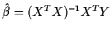 to
get
to
get
![\begin{displaymath}\hat\beta = \left[\begin{array}{c}
\bar{Y} \\
(X_1^TX_1)^{-1...
...0 \\
\tilde\beta_1 \\
\tilde\beta_2
\end{array}\right] \, .
\end{displaymath}](img64.gif)
- (e)
- Let
 be the vectors of fitted values corresponding to the
estimates
be the vectors of fitted values corresponding to the
estimates
 for i=1,2,3. [Note this should be 0,1,2]
Show that for
for i=1,2,3. [Note this should be 0,1,2]
Show that for  we have
 .
.
Solution

because the centre term X1TX2=0. You must check similar formulas for and so on.
- (f)
- For the design matrix Xb of the first assignment identify
X1 and X2 and verify the orthogonality condition of this
problem.
Solution
In the solution set for assignment the first column of Xbis 1, the second is X1 and the other two columns are X2. Now just multiply things like X1T X2 to make sure you get 0.
Solution
I used the following SAS code to find the mean age and to compute the correlation between age and age cubed:
data product;
 infile "CH07PR33.DAT";
 input product age;
proc means ;
proc glm;
  model age = age*age*age;
run;
Part of the output is
Variable   N          Mean       Std Dev       Minimum       Maximum
--------------------------------------------------------------------
PRODUCT   18   104.2222222     5.4292839    93.0000000   112.0000000
AGE       18    40.0000000    13.2842233    20.0000000    60.0000000
--------------------------------------------------------------------

Dependent Variable: AGE
                               Sum of          Mean
Source              DF        Squares        Square  F Value    Pr > F
Model                1     2799.13108    2799.13108   222.96    0.0001
Error               16      200.86892      12.55431
Corrected Total     17     3000.00000
              R-Square           C.V.      Root MSE           AGE Mean
              0.933044       8.858015       3.54321            40.0000

                               T for H0:     Pr > |T|    Std Error of
Parameter        Estimate     Parameter=0                  Estimate

INTERCEPT     24.61714029           18.56      0.0001      1.32618815
AGE*AGE*AGE    0.00018313           14.93      0.0001      0.00001226
Since
r2 = 0.933 and the slope is positive we find that the correlation between
age and age cubed is 0.966.
Having found the mean age I did the rest of the problem with:
data product;
 infile "CH07PR33.DAT";
 input product age;
 agec = age-40;
 agec2 = agec*agec;
 agec3 = agec*agec*agec;
proc print;
proc glm;
  model product= agec agec2 agec3;
output out=prodout r=resid p=fitted ;
run;
proc glm;
  model agec3 = agec;
run;
proc rank normal=vw data=prodout out=prodout2;
  var resid;
  ranks normscr;
run;
proc gplot data=prodout2;
 plot resid*agec;
 plot resid*fitted;
 plot resid*normscr;
run;
obtaining the (edited) output:
              OBS    PRODUCT    AGE    AGEC    AGEC2    AGEC3
                1       97       20     -20     400     -8000
                2       93       20     -20     400     -8000
                3       99       25     -15     225     -3375
                4      105       25     -15     225     -3375
                5      109       30     -10     100     -1000
                6      106       30     -10     100     -1000
                7      109       35      -5      25      -125
                8      111       35      -5      25      -125
                9      100       40       0       0         0
               10      105       40       0       0         0
               11       97       45       5      25       125
               12      101       45       5      25       125
               13      105       50      10     100      1000
               14      103       50      10     100      1000
               15      105       55      15     225      3375
               16      109       55      15     225      3375
               17      112       60      20     400      8000
               18      110       60      20     400      8000

Dependent Variable: PRODUCT
                               Sum of          Mean
Source              DF        Squares        Square  F Value    Pr > F
Model                3     351.680014    117.226671    10.98    0.0006
Error               14     149.431097     10.673650
Corrected Total     17     501.111111

              R-Square           C.V.      Root MSE       PRODUCT Mean
              0.701800       3.134701       3.26706            104.222

Source              DF      Type I SS   Mean Square  F Value    Pr > F
AGEC                 1     124.033333    124.033333    11.62    0.0042
AGEC2                1       2.955267      2.955267     0.28    0.6070
AGEC3                1     224.691414    224.691414    21.05    0.0004

Source              DF    Type III SS   Mean Square  F Value    Pr > F
AGEC                 1      92.201230     92.201230     8.64    0.0108
AGEC2                1       2.955267      2.955267     0.28    0.6070
AGEC3                1     224.691414    224.691414    21.05    0.0004


                             T for H0:     Pr > |T|    Std Error of
Parameter      Estimate     Parameter=0                  Estimate
INTERCEPT   104.6839827           89.66      0.0001      1.16751237
AGEC         -0.4591751           -2.94      0.0108      0.15623072
AGEC2        -0.0027706           -0.53      0.6070      0.00526534
AGEC3         0.0022458            4.59      0.0004      0.00048948

Dependent Variable: AGEC3
                               Sum of          Mean
              R-Square           C.V.      Root MSE         AGEC3 Mean
              0.854233        9999.99       1668.64                  0

                             T for H0:     Pr > |T|    Std Error of
Parameter      Estimate     Parameter=0                  Estimate
INTERCEPT     0.0000000            0.00      1.0000     393.3033181
AGEC        295.0000000            9.68      0.0001      30.4651440
We are now in a position to answer the individual questions.
- 7.33 a)
- The coefficients are in the print-out. Multiple
R2 =
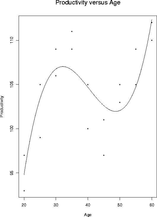
0.702. Here is a plot, in SPlus, of the data and fitted values. It is
adequate, more or less, although there is a sense that the cubic is
too low around 35 years of age and too high around 45. There is a danger of
overinterpretation, however.
- b)
- This question asks you to test
 ,
against the alternative that at least one of these coefficients is not 0.
The overall F test does exactly this: F=10.98 and P=0.006 Since P<0.01you would reject at the 1% level. The conclusion is that there is some
relation between age and productivity.
,
against the alternative that at least one of these coefficients is not 0.
The overall F test does exactly this: F=10.98 and P=0.006 Since P<0.01you would reject at the 1% level. The conclusion is that there is some
relation between age and productivity.
- e)
- The fitted regression function is

You can expand out the powers if you want but it's not really useful. The correlation between Age and Age cubed is 0.966 while that between centered age and centered age cubed is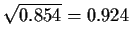 which makes the
centering not very useful for decreasing the correlation between
which makes the
centering not very useful for decreasing the correlation between
 and
and
 .
However, the centering is more
numerically stable and lowers the correlation between x
and x3 quite a bit.
.
However, the centering is more
numerically stable and lowers the correlation between x
and x3 quite a bit.
- 7.34a
- To carry out this test you need to compare the linear model
with this cubic model. This can be done by rerunning SAS with the model
statement model product=agec but you can also do it with the output
above. The Type I SS table shows the extra sums of squares for comparing
a sequence of models:
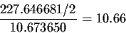
Model ESS cubic 149.431097 quadratic 149.431097 + 224.691414 =374.122511 linear 374.122511 + 2.955267 The extra sum of squares due to quadratic and cubic terms is then the sum of the last two lines in the Type I SS table which is 227.646681. There are two more parameters in the cubic model than in the linear model so there are 2 degrees of freedom for the extra SS. The F statistic is
on 2, 14 degrees of freedom. (The denominator is just the MSE for the cubic model.) You would need to use F tables to decide whether or not to reject. In fact P is about 0.0015 so you cannot discard the quadratic and cubic terms. - b)
- This can be done using the last line of either the Type 1 or Type
3 SS tables since these lines both compare the cubic and quadratic models.
The F statistic is 21.05 with a P value of 0.0004 so you definitely
cannot drop the cubic term. Null is
 ,
alternative is
,
alternative is
 and the conclusion is that
.
and the conclusion is that
.
- 7.35 a)
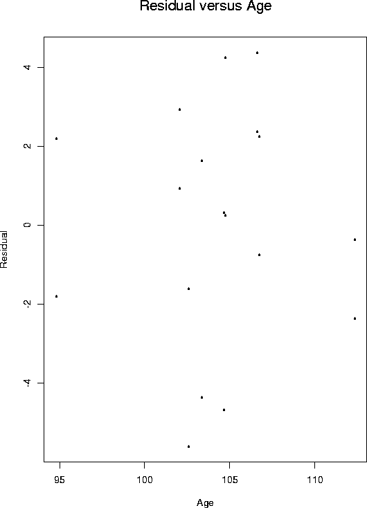
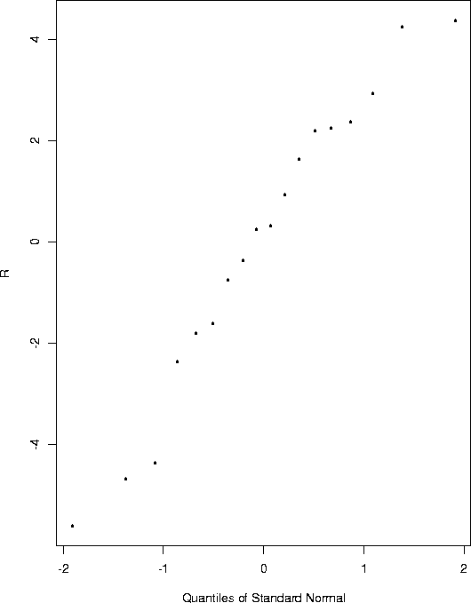
- The plots are prepared by the SAS code above. Here
are the SPlus versions. They were prepared with the following SPlus
code:
#
# Read in the data into a matrix (technically
# a data frame)
#
data <- read.table("CH07PR33.DAT")
#
# Add a new column to the matrix which has the Ages minus
# the mean age
#
data <- cbind(data,data[,2]-mean(data[,2]))
#
# Give names to the variables in the data frame
#
names(data) <- c("Product","Age","AgeCen")
#
# Compute the mean age for later use
#
m <- mean(data$Age)
#
# make the variables in the data frame available for general
# use without having to say things like data$Age
# which names the Age component of the data frame called data
#
attach(data)
#
# Regress the variable Product on the first three
# powers of the centered Age. Keep the results of
# the regression in a variable called fit
#
fit <- lm( Product ~ AgeCen+AgeCen^2 + AgeCen^3,data=data)
#
# store the residuals in R
#
R <- resid(fit)
#
# store the fitted values in Fit
Fit <- predict(fit)
#
#  Make a postscript plot in a file fit.ps. The horizontal=F
# causes the image to be in portrait orientation, that is,
# in the usual direction (not turned sideways) on a piece
# of paper.
#
postscript("fit.ps",horizontal=F)
#
#  Plot Productivity versus Age.
#
plot(Age, Product,xlab="Age", ylab="Productivity",
   main="Productivity versus Age")
#
# Add a plot of the fitted cubic
#
# First make a vector full of ages
#
xp <- seq(from=min(Age),to=max(Age),length=500)
#
# now compute the corresponding fitted values
# The regression coefficients are obtained using
# the function coef.
#
co <- coef(fit)
yp <- co[1] + co[2]*(xp-m)
        + co[3]*(xp-m)^2 + co[4]*(xp-m)^3
#
# Add a curve to the plot
#
lines(xp,yp)
#
# finish this plot
#
dev.off()

#
# Now plot residuals against Fitted value
#
postscript("r_v_fit.ps",horizontal=F)
plot(Fit,R,xlab="Fitted Value",
        ylab="Residual",main="Residual versus Fitted Value")
dev.off()
#
# Now plot residuals against Age
#
postscript("r_v_age.ps",horizontal=F)
plot(Fit,R,xlab="Age",ylab="Residual",main="Residual versus Age")
dev.off()
#
# Make a QQ plot
#
postscript("qq.ps",horizontal=F)
qqnorm(R)
dev.off()