Postscript version of these questions

STAT 350

Assignment 5

Part A

1.

In this question you will derive some of the formulas for case deleted statistics. Suppose that X is an $n\times p$ design matrix. Let x_i^T be the $i^{\mbox{th}}$ row of X (so that, x_i is a column vector or dimension p). Let X_(i) be the design matrix with case ideleted and Y_(i) the vector of n-1 responses with case ideleted.

(a)

Use partitioned matrices to show

$$X_{(i)}^T Y_{(i)} = X^TY -x_iY_i \, .$$

Write

$$X = \left[\begin{array}{r} x_1^T \\ x_2^T\\ \vdots \\ x_n^T \end{array}\right]$$

and

$$Y = \left[\begin{array}{r} Y_1 \\ Y_2\\ \vdots \\ Y_n \end{array}\right]$$

Then

$$X^TY = \left[x_1 \vert x_2 \vert \cdots \vert x_n\right] \lef... ... Y_2\\ \vdots \\ Y_n \end{array}\right] = \sum_{j=1}^n x_j Y_j$$

Since X_(i) and Y_(i) simply omit the ith rows we see

$$X_{(i)}^T Y_{(i)} = X^TY -x_iY_i \, .$$

(b)

Show

$$X_{(i)}^TX_{(i)} = X^TX - x_ix_i^T \, .$$

We have

$$X^TX = \left[x_1 \vert x_2 \vert \cdots \vert x_n\right] \lef... ...T\\ \vdots \\ x_n^T \end{array}\right] = \sum_{j=1}^n x_jx_j^T$$

Again omitting the ith term we find

$$X_{(i)}^TX_{(i)} = X^TX - x_ix_i^T \, .$$

(c)

Suppose B is an invertible symmetric $p\times p$ matrix and v is a column vector of dimension p. Show, by direct multiplication, that (B-vv^T)^-1 is of the form

B^-1 + r B^-1vv^T B^-1

and give a formula for the scalar r.

Simply multiply

(B-vv^T)(B^-1 +r B^-1vv^T B^-1) = I + r vv^T B^-1 - vv^T B^{- 1} - r vv^T B^-1vv^T B^-1

The trick most students missed is that in the last term the quantity v^T B^-1v is a scalar, that is, just a single number (check that it is a $1\times 1$ matrix). It may help to give it a name like s to see that the last term is

$$rs vv^TB^{-1} \, .$$

Thus

(B-vv^T)(B^-1 +r B^-1vv^T B^-1) = I + (r -1 -rs)vv^T B^-1

which is the identity matrix if

$$r-rs -1 = 0 \, .$$

Solving gives r=1/(1-s) = 1/(1-v^TB^-1v). Many students got a formula like

r = (1-vv^TB^-1)^-1

which is a $p\times p$ matrix not a scalar.

(d)

Apply to previous part to show

(X_(i)^TX_(i))^-1 = (X^TX)^-1 + r_i(X^TX)^-1 x_i x_i^t (X^TX)^-1

and give a formula for r_i in terms of the leverage h_ii = x_i^T (X^TX)^-1 x_i.

Put B=X^TX and v=x_i. You get

r_i = 1/(1-x_i^T (X^TX)^-1 x_i) = 1/(1-h_ii)

and

$$(X_{(i)}^TX_{(i)})^{-1} = (X^TX)^{-1} + r_i (X^TX)^{-1} x_i x_i^T (X^TX)^{-1}\, .$$

(e)

Show 1+h_iir_i = r_i.

We have

$$(1+r_i h_{ii}) = \frac{1-h_{ii}}{1-h_{ii}} + \frac{h_{ii}}{1-h_{ii}} = \frac{1}{1-h_{ii}} = r_i$$

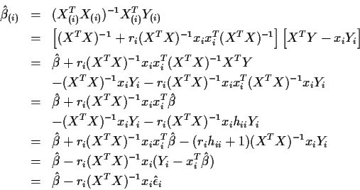
(f)

Show that

$$\begin{eqnarray*}\hat\beta_{(i)} & = & \hat\beta +r_i (X^TX)^{-1} x_i x_i^T \hat... ...i \\ & = & \hat\beta - r_i (X^TX)^{-1} x_i \hat\epsilon_i \, . \end{eqnarray*}$$

$$\begin{eqnarray*}\hat\beta_{(i)} & = & (X_{(i)}^TX_{(i)})^{-1}X_{(i)}^T Y_{(i)} ... ...t\beta) \\ & = & \hat\beta - r_i (X^TX)^{-1} x_i \hat\epsilon_i \end{eqnarray*}$$

(g)

Deduce that $\hat\mu_{(i)} = \hat\mu_i - r_i h_{ii} \hat\epsilon_i$.

Multiply $\hat\beta_{(i)}$ by x_i to get

$$\hat\mu_{(i)} = \hat\mu -r_i x_i (X^TX)^{-1} x_i \hat\epsilon_i =\hat\mu -r_i h_{ii} \hat\epsilon_i$$

(h)

Show that the $i^{\mbox{th}}$ PRESS residual $Y_i - \hat\mu_{(i)}$ is given by

$$Y_i - \hat\mu_{(i)} = r_i\hat\epsilon_i \,$$

$$PRESS_i = Y_i - \hat\mu_{(i)} = Y_i -\hat\mu_i + r_i h_{ii } ... ...\epsilon_i = (1+r_i h_{ii}) \hat\epsilon_i = r_i\hat\epsilon_i$$

(i)

Derive the formula for the $i^{\mbox{th}}$externally studentized (case deleted) residual.

The variance of the PRESS residual is $Var(r_i\hat\epsilon_i) = \sigma^2 r_i^2 (1-h_{ii}) =\sigma^2 r_i$. The externally studentized residual is the PRESS residual divided by an estimate of its standard error where $\sigma^2$ is estimated by MSE_(i). Thus the externally studentized residual is

$$\frac{PRESS_i}{\sqrt{MSE_{(i)} r_i}} = \frac{\hat\epsilon_i ... ...{(i)}} } = \frac{\hat\epsilon_i}{\sqrt{MSE_{(i)} (1-h_{ii})}}$$

To get the simplest formula we must actually simplify MSE_(i).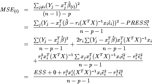

$$\begin{eqnarray*}MSE_{(i)} & = & \frac{\sum_{j \neq i} (Y_j - x_j^T \hat\beta_{... ...(X^TX)^{-1} x_i\hat\epsilon_i^2 - r_i^2 \hat\epsilon_i^2}{n-p-1} \end{eqnarray*}$$

The middle term vanishes because

$$\sum (Y_j - x_j^T\hat\beta)x_j = X^TY-X^TX\hat\beta=0\,.$$

Use r_i²(1-h_ii)=r_i to get

$$MSE_{(i)} = \frac{ESS - r_i \hat\epsilon_i^2}{n-p-1}$$

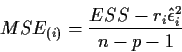
and then you can deduce the final formula given in class.

2.

For the Nitrogen Output in Wallabies data set from Assignment 3 do forward, backward, stepwise and all subsets regression.

Here is code for all the methods and with all subsets done both using C_p and using adjusted R².

data nit;
  infile 'nit.dat' ;
  input nitexc weight dryin wetin nitin ;
proc reg  data=nit;
   model nitexc = weight dryin wetin 
         nitin /selection=FORWARD;
run ;
proc reg  data=nit;
   model nitexc = weight dryin wetin 
         nitin /selection=BACKWARD;
run ;
proc reg  data=nit;
   model nitexc = weight dryin wetin 
         nitin /selection=STEPWISE;
run ;
proc reg  data=nit;
   model nitexc = weight dryin wetin 
         nitin /selection=CP;
run ;
proc reg  data=nit;
   model nitexc = weight dryin wetin 
         nitin /selection=ADJRSQ;
run ;

The conclusion of the output is that BACKWARD and STEPWISE settle for the model containing only Nitrogen Intake as a predictor. The forward selection method also includes Wet Intake because of the very high level of $\alpha$ (0.5) to enter. The all subsets method using C_p would settle on the model using only nitrogen intake but the adjusted R² method also includes Wet Intake. However, overall there seems little reason to include Wet Intake since it improves the fit very little and is not very significant at all.

3.

Problem 23.12, 23.13 parts c,d,e,f,g only and 23.14.

Here is code for the analysis of variance.

options pagesize=60 linesize=80;
data electron;
 infile 'anova.dat' firstobs=2;
 input Time Sex Sequence Exper Replic;
proc glm  data=electron;
 class Sex Sequence Exper ;
 model time = Sex|Sequence|Exper ;
 means sex sequence exper sex*sequence*exper;
 estimate 'sexdif' sex 1 -1;
 estimate 'seq12dif' sequence 1 -1 0;
 estimate 'seq13dif' sequence 1 0 -1;
 estimate 'seq23dif' sequence 0 1 -1;
 estimate 'expdif' exper 1 -1;
 output out=anovres r=resid;
proc rank data=anovres normal=blom out=ressc;
 var resid;
 ranks nscores;
proc corr data=ressc;
 var resid nscores;
run;

COMMENTS

• You use the class statement to let SAS know that the factors are categorical.

• The model statement requests that all two way and the three way interaction terms be fitted.

• The means statement computes means and standard deviations for the groups defined by the levels of sex, of sequence, of exper and of all the 3 way combinations.

• The estimate statements compute the differences in means between the two sexes, between the 1st and second sequence, the first and third sequence and between the two levels of experience. This hinges on the use of a balanced design.

• The proc rank statements compute approximations to the expected values of normal order statistics needed for the correlation test in 23.12b.

• The correlation is actually computed by proc corr.

The complete output.

You can read the type III sums of squares table to do F tests without doing multiple runs because each effect has a sum of squares which is unaffected by the presence of the others. The conclusion is that the three way interaction is insignificant and all three two way interactions are insignificant. All three main effects are significant; none can be eliminated.

In the question on Bonferroni confidence intervals the 5 quantities to be estimated are each estimated by a difference of two averages so that the variance of the estimated difference is of the form

$$\sigma^2 (\frac{1}{n_1}+\frac{1}{n_2})$$

You work out standard t type confidence intervals by estimating the means as usual (see the means statment) and replacing $\sigma^2$ by the MSE in the formula for the variance. The Bonferroni method just replaces the $\alpha$ of 0.01 by $\alpha/5 = 0.02$ for 5 confidence intervals. The t critical value is t_0.02/2,48= 2.41. For the sex difference for instance the average time for men is 1155.933 seconds while for women it is 966.1333. The difference is 189.8 and this is computed by the means statement whose output is

                      T for H0:   Pr>|T| Std Error of
Parameter   Estimate Parameter=0          Estimate
sexdif    189.800000    25.10     0.0001  7.56325180
seq12dif  -57.250000    -6.18     0.0001  9.26305385
seq13dif    6.600000     0.71     0.4796  9.26305385
seq23dif   63.850000     6.89     0.0001  9.26305385
expdif    159.666667    21.11     0.0001  7.56325180

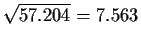Notice the standard errors. The mean squared error in the model is 858.06. There are 30 men and 30 women so the variance of the difference between men's average and women's average is 858.06(1/30+1/30) = 57.204. The standard error of the estimate of $\mu_{1\cdot\cdot} -\mu_{2\cdot\cdot}$ is then $\sqrt{57.204} = 7.563$ as in the output. The desired confidence intervals are all and estimate from the column labelled Estimate plus or minus 2.41 times a standard error from the last column.

The needed mean for $\hat\mu_{231}$ is produced by means. The key point is that the standard error to attach to the mean is $\sqrt{MSE/5}$ which is based on 48 degrees of freedom, not on 4.

4.

Problem 25.11 parts a, b anc c, 25.12 part c.

For this question I used the SAS code

data knees;
  infile 'knees.dat' firstobs=2;
  input Days Fitness Patient Age ;
proc glm  data=knees;
  class Fitness ;
  model Days = Fitness|Age ;
proc glm  data=knees;
  class Fitness ;
  model Days = Fitness Age ;
  output out=anovres r=resid p=fitted;
proc rank data=anovres normal=blom out=ressc;
  var resid;
  ranks nscores;
proc corr data=ressc;
  var resid nscores;
proc print data=ressc;
  var fitted fitness age resid nscores;
run;

getting the output ( complete output )

                        General Linear Models Procedure
Dependent Variable: DAYS   
                       Sum of        Mean
Source        DF      Squares      Square F Value Pr > F
Model          5 1082.0560870 216.4112174  655.36 0.0001
Error         18    5.9439130   0.3302174
Correctd Totl 23 1088.0000000
        R-Square         C.V.      Root MSE  DAYS Mean
        0.994537     1.795767     0.5746454  32.000000
Source      DF  Type III SS   Mean Square F Value Pr > F
FITNESS      2   5.44989183    2.72494592    8.25 0.0029
AGE          1 369.44147783  369.44147783 1118.78 0.0001
AGE*FITNESS  2   0.22183487    0.11091744    0.34 0.7191

                        General Linear Models Procedure
Dependent Variable: DAYS   
                       Sum of        Mean
Source        DF      Squares      Square F Value Pr > F
Model          3 1081.8342521 360.6114174 1169.72 0.0001
Error         20    6.1657479   0.3082874
Correctd Totl 23 1088.0000000
    R-Square         C.V.      Root MSE      DAYS Mean
    0.994333     1.735114     0.5552363      32.000000
Source  DF  Type III SS   Mean Square F Value   Pr > F
FITNESS  2 246.08370505  123.04185252  399.11   0.0001
AGE      1 409.83425209  409.83425209 1329.39   0.0001

                    Correlation Analysis
          Pearson Correlation Coefficients 

                      RESID  
       NSCORES      0.99488 

 OBS     FITTED    FITNESS     AGE      RESID      NSCORES

   1    28.7930       1       18.3     0.20697     0.26136
   2    42.4503       1       30.0    -0.45028    -0.87524
   3    38.3648       1       26.5    -0.36478    -0.60318
   4    40.2324       1       28.1    -0.23244    -0.48332
   5    42.1001       1       29.7     0.89991     1.94690
   6    39.8822       1       27.8     0.11775     0.05171
   7    30.5440       1       19.8    -0.54396    -1.03865
   8    41.6332       1       29.3     0.36682     0.73241
   9    29.8639       2       20.8     0.13613     0.15568
  10    34.9999       2       25.2     0.00007    -0.05171
  11    39.6691       2       29.2    -0.66907    -1.23590
  12    28.9300       2       20.0    -0.93004    -1.49843
  13    30.6810       2       21.5     0.31903     0.60318
  14    31.3813       2       22.1    -0.38134    -0.73241
  15    28.5799       2       19.7     0.42015     0.87524
  16    34.4163       2       24.7     0.58372     1.03865
  17    29.1635       2       20.2    -0.16349    -0.26136
  18    32.3152       2       22.9     0.68483     1.23590
  19    25.2062       3       22.7     0.79380     1.49843
  20    32.2099       3       28.7    -0.20991    -0.37006
  21    20.7705       3       18.9     0.22949     0.37006
  22    19.7199       3       18.0     0.28005     0.48332
  23    24.0389       3       21.7    -1.03891    -1.94690
  24    22.0545       3       20.0    -0.05452    -0.15568

For part a of 25.11 the residuals are printed out above. For part b the plots desired are:

The conclusion is that neither the residual plots nor the Q-Q plot show any major problems.

For part c, the generalized model is

$$Y_{ij} = \mu + \tau_i + \gamma_i(x_{ij}-\bar{x}_{\cdot\cdot}) +\epsilon_{ij}$$

and the null hypothesis is that all the $\gamma_i$ are equal. This is tested by comparing the two model statements model days = fitness | age and model days = fitness age, doing an extra sum of squares F test. The resulting F statistic is the Type III sum of squares for fitness*age giving F=0.34 and P=0.7191. The null hypothesis is accepted.

For 25.12 part c the F statistic is obtained from the Type III sum of squares for fitness for the model days = fitness age statement. This has F=399.11 and P=0.0001There is clearly an effect of the variable Fitness.

The estimate statements permit us to compare the three levels of fitness. SAS prints out estimates of the differences in the intercepts. The relevant output is

                              T for H0: Pr>|T| Std Err of
Parameter           Estimate  Param=0            Estimate
High v Low Fitness -8.72289277 -26.20   0.0001 0.33296397
High v Med Fitness -6.87551411 -23.84   0.0001 0.28837673
Med  v Low Fitness -1.84737866  -6.44   0.0001 0.28694289

Notice that the fit group appears to recuperate about 9 days faster than the unfit group!