Postscript version of this file

STAT 801 Lecture 1

Course outline

Reading for Today's Lecture: Chapter 1 of Casella and Berger.

Goals of Today's Lecture:

• Give an overview of the course.

• Define
  • Probability Space

  • Random variables (in R^p)

  • The distribution of a random variable

  • Cumulative Distribution Function (in R¹)

  • Discrete and Absolutely Continuous Distribution

  • Probability Mass Function

  • Probability Density

• Introduce the problem of distribution theory.

Today's notes

Course outline:

• Distribution Theory. Chapters 1 through 5 of Casella and Berger (but Chapter 3 will be regarded as review and not covered in class).
  • Basic concepts of probability.

  • Distributions

  • Expectation and moments

  • Transforms (characteristic functions, moment generating functions)

  • Distribution of transformations

• Point estimation (Chapters 6 and 7 in Casella and Berger.)
  • Maximum likelihood estimation.

  • Method of moments.

  • Optimality Theory.

  • Bias, mean squared error.

  • Sufficiency.

  • Uniform Minimum Variance Unbiased Estimators.

• Hypothesis Testing (Cf. Chapter 8 in Casella and Berger.)
  • Neyman Pearson optimality theory.

  • Most Powerful, Uniformly Most Powerful, Unbiased tests.

• Confidence sets (Cf. Chapter 9 in Casella and Berger.)
  • Pivots

  • Associated Hypothesis Tests

  • Inversion of hypothesis tests to get confidence sets.

• Decision Theory. (Cf. Chapter 10 in Casella and Berger.)

Statistics versus Probability

Standard view of scientific inference has a set of theories which make predictions about the outcomes of an experiment:

Theory	Prediction
A	1
B	2
C	3

If we conduct the experiment and see outcome 2 we infer that Theory B is correct (or at least that A and C are wrong).

Add Randomness

Theory	Prediction
A	Usually 1 sometimes 2 never 3
B	Usually 2 sometimes 1 never 3
C	Usually 3 sometimes 1 never 2

Now if we actually see outcome 2 we infer that Theory B is probably correct, that Theory A is probably not correct and that Theory C is wrong.

Probability Theory is concerned with constructing the table just given: computing the likely outcomes of experiments.

Statistics is concerned with the inverse process of using the table to draw inferences from the outcome of the experiment. How should we do it and how wrong are our inferences likely to be?

Probability Definitions

A Probability Space (sometimes called a Sample Space) is an ordered triple $(\Omega, {\cal F}, P)$. The idea is that $\Omega$ is the set of possible outcomes of a random experiment, $\cal F$ is the set of those events, or subsets of $\Omega$ whose probability is defined and P is the rule for computing probabilities. Formally:

• $\Omega$ is a set.

• $\cal F$ is a family of subsets of $\Omega$ with the property that $\cal F$ is a $\sigma$-field (or Borel field or $\sigma$-algebra):

  1.

  The empty set $\emptyset$ and $\Omega$ are members of $\cal F$.

  2.

  $\cal F$ is closed under complementation. That is, if A is in $\cal F$ (meaning P(A) is defined) then $A^c =\{\omega\in\Omega: \omega \not\in A\}$ is in $\cal F$ (because we want to be able to say P(A^c)=1-P(A))>

  3.

  If $A_1,A_2,\cdots$ are all in $\cal F$ then so is $A = \cup_{i=1}^\infty A_i$. (A is the event that at least one of the A_i happens and we want to be sure that if each of the A_i has a probability then so does this event A.)

• P is a function whose domain is $\cal F$ and whose range is a subset of [0,1] which satisfies the axioms for a probability:

  1.

  $P(\emptyset)=0$ and $P(\Omega)=1$.

  2.

  If $A_1,A_2,\cdots$ are pairwise disjoint (or mutually exclusive) ( meaning for any $j\neq k$ $A_j\cap A_k=\emptyset$) then
  

  $$P(\cup_{i=1}^\infty A_i) = \sum_{i=1}^\infty P(A_i)$$

  
  

  This property is called countable additivity.

These axioms guarantee that as we compute probabilities by the usual rules, including approximation of an event by a sequence of others we don't get caught in any logical contradictions.

A vector valued random variable is a function X whose domain is $\Omega$ and whose range is in some p dimensional Euclidean space, R^p with the property that the events whose probabilities we would like to calculate from their definition in terms of X are in $\cal F$. We will write $X=(X_1,\ldots,X_p)$. We will want to make sense of

$$P(X_1 \le x_1, \ldots , X_p \le x_p)$$

for any constants $(x_1,\ldots,x_p)$. In our formal framework the notation

$$X_1 \le x_1, \ldots , X_p \le x_p$$

is just shorthand for an event, that is a subset of $\Omega$, defined as

$$\left\{\omega\in\Omega: X_1(\omega) \le x_1, \ldots , X_p (\omega) \le x_p \right\}$$

Remember that X is a function on $\Omega$ so that X₁ is also a function on $\Omega$. In almost all of probability and statistics the dependence of a random variable on a point in the probability space is hidden! You almost always see X not $X(\omega)$.

Now for formal definitions:

The Borel $\sigma$-field in R^p is the smallest $\sigma$-field in R^p containing every open ball.

Every common set is a Borel set, that is, in the Borel $\sigma$-field

An R^p valued random variable is a map $X:\Omega\mapsto R^p$ such that when A is Borel then $\{\omega\in\Omega:X(\omega)\in A\} \in \cal F$.

Fact: this is equivalent to

$$\left\{ \omega\in\Omega: X_1(\omega) \le x_1, \ldots , X_p (\omega) \le x_p \right\} \in \cal F$$

for all $(x_1,\ldots,x_p)\in R^p$.

Jargon and notation: we write $P(X\in A)$ for $P(\{\omega\in\Omega:X(\omega)\in A)$ and define the distribution of X to be the map

$$A\mapsto P(X\in A)$$

which is a probability on the set R^p with the Borel $\sigma$-field rather than the original $\Omega$ and $\cal F$.

The Cumulative Distribution Function (or CDF) of X is the function F_X on R^p defined by

$$F_X(x_1,\ldots, x_p) = P(X_1 \le x_1, \ldots , X_p \le x_p)$$

Properties of F_X (or just F when there's only one cdf under consideration):

1.

$0 \le F(x) \le 1$.

2.

$x> y \Rightarrow F(x) \ge F(y)$ (F is monotone non-decreasing).

3.

$\lim_{x\to - \infty} F(x) = 0$

4.

$\lim_{x\to \infty} F(x) = 1$

5.

$\lim_{x\searrow y} F(x) = F(y)$ (F is right continuous).

6.

$\lim_{x\nearrow y} F(x) \equiv F(y-)$ exists.

7.

F(x)-F(x-) = P(X=x).

8.

F_X(t) = F_Y(t) for all t implies that X and Y have the same distribution, that is, $P(X\in A) = P(Y\in A)$ for any (Borel) set A.

The distribution of a random variable X is discrete (we also call the random variable discrete) if there is a countable set $x_1,x_2,\cdots$ such that

$$P(X \in \{ x_1,x_2 \cdots\}) =1 = \sum_i P(X=x_i)$$

In this case the discrete density or probability mass function of X is

f_X(x) = P(X=x)

The distribution of a random variable X is absolutely continuous if there is a function f such that

$$P(X\in A) = \int_A f(x) dx$$

for any (Borel) set A. This is a p dimensional integral in general. This condition is equivalent to

$$F(x) = \int_{-\infty}^x f(y) \, dy$$

We call f the density of X. For most values of x we then have F is differentiable at x and

$$F^\prime(x) =f(x) \, .$$

Example: X is exponential.

$$F(x) = \left\{ \begin{array}{ll} 1- e^{-x} & x > 0 \\ 0 & x \le 0 \end{array}\right.$$

$$f(x) = \left\{ \begin{array}{ll} e^{-x} & x> 0 \\ \mbox{undefined} & x= 0 \\ 0 & x < 0 \end{array}\right.$$

Distribution Theory

General Problem: Start with assumptions about the density or cdf of a random vector $X=(X_1,\ldots,X_p)$. Define $Y=g(X_1,\ldots,X_p)$ to be some function of X (usually some statistic of interest). How can we compute the distribution or cdf or density of Y?

Univariate Techniques

Method 1: compute the cdf by integration and differentiate to find f_Y.

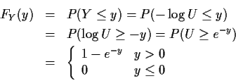
Example: $U \sim \mbox{Uniform}[0,1]$ and $Y=-\log U$. Then

$$\begin{eqnarray*}F_Y(y) & = & P(Y \le y) = P(-\log U \le y) \\ & = & P(\log U ... ...{array}{ll} 1- e^{-y} & y > 0 \\ 0 & y \le 0 \end{array}\right. \end{eqnarray*}$$

so that Y has a standard exponential distribution.

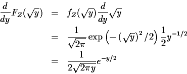
Example: $Z \sim N(0,1)$, i.e.

$$f_Z(z) = \frac{1}{\sqrt{2\pi}} e^{-z^2/2}$$

and Y=Z². Then

$$F_Y(y) = P(Z^2 \le y) = \left\{ \begin{array}{ll} 0 & y < ... ... P(-\sqrt{y} \le Z \le \sqrt{y}) & y \ge 0 \end{array}\right.$$

Now

$$P(-\sqrt{y} \le Z \le \sqrt{y}) = F_Z(\sqrt{y}) -F_Z(-\sqrt{y})$$

can be differentiated to obtain

$$f_Y(y) = \left\{ \begin{array}{ll} 0 & y < 0 \\ \frac{d}{dy... ...\right] & y > 0 \\ \mbox{undefined} & y=0 \end{array}\right.$$

Then

$$\begin{eqnarray*}\frac{d}{dy} F_Z(\sqrt{y}) & = & f_Z(\sqrt{y})\frac{d}{dy}\sqrt... ...frac{1}{2} y^{-1/2} \\ & = & \frac{1}{2\sqrt{2\pi y}} e^{-y/2} \end{eqnarray*}$$

with a similar formula for the other derivative. Thus

$$f_Y(y) = \left\{ \begin{array}{ll} \frac{1}{\sqrt{2\pi y}} e... ...0 \\ 0 & y < 0 \\ \mbox{undefined} & y=0 \end{array}\right.$$

We will find indicator notation useful:

$$1(y>0) = \left\{ \begin{array}{ll} 1 & y>0 \\ 0 & y \le 0 \end{array}\right.$$

which we use to write

$$f_Y(y) = \frac{1}{\sqrt{2\pi y}} e^{-y/2} 1(y>0)$$

(changing the definition unimportantly at y=0).

Notice: I never evaluated F_Y before differentiating it. In fact F_Y and F_Z are integrals I can't do but I can differentiate then anyway. You should remember the fundamental theorem of calculus:

$$\frac{d}{dx} \int_a^x f(y) \, dy = f(x)$$

at any x where f is continuous.