![]()
![]()
![]()
Reading for Today's Lecture: Chapters 1, 2 and 4 of Casella and Berger.
Goals of Today's Lecture:
Today's notes
So far we have defined probability space, real and vector valued random variables cumulative distribution functions in R1 and Rp, discrete densities and densities for random variables with absolutely continuous distributions.
We also started distribution theory. So far: for Y=g(X) with X and Y
each real valued
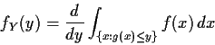
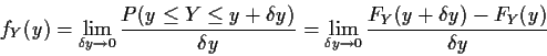
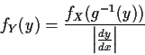
Method 2: Change of variables.
Now assume g is one to one.
I will do the case where g is increasing
and I will be assuming that g is differentiable.
The density has the following interpretation (mathematically
what follows is just the expression of the fact that
the density is the derivative of the cdf):
Remark: If g had been decreasing the derivative ![]() would
have been negative but in the argument above the interval
would
have been negative but in the argument above the interval
![]() would have to have been written in the other order. This would have meant that
our formula had
would have to have been written in the other order. This would have meant that
our formula had
![]() .
In both
cases this amounts to the formula
.
In both
cases this amounts to the formula
Example:
![]() or
or
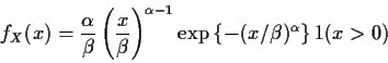
Let ![]() so that
so that
![]() .
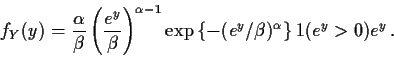
Setting
.
Setting ![]() and solving
gives
and solving
gives ![]() so that
g-1(y) = ey. Then
so that
g-1(y) = ey. Then
![]() and
and
![]() .
Hence
.
Hence
Now we turn to multivariate problems. The simplest version has
![]() and Y=X1 (or in general any Xj).
and Y=X1 (or in general any Xj).
We call
![]() the marginal density of
the marginal density of
![]() and use the
expression joint density for fX but
and use the
expression joint density for fX but
![]() is exactly the
usual density of
is exactly the
usual density of
![]() .
The adjective ``marginal'' is just there to
distinguish the object from the joint density of X.
.
The adjective ``marginal'' is just there to
distinguish the object from the joint density of X.
Example The function
The general multivariate problem has
Case 1: If q>p then Y will not have a density for ``smooth'' g. Y will have a singular or discrete distribution. This sort of problem is rarely of real interest. (However, variables of interest often have a singular distribution - this is almost always true of the set of residuals in a regression problem.)
Case 2 If q=p then we will be able to use a change of variables formula which generalizes the one derived above for the case p=q=1. (See below.)
Case 3: If q < p we will try a two step process.
In the first step we pad out Y
by adding on p-q more variables (carefully chosen)
and calling them
![]() .
Formally we find functions
.
Formally we find functions
![]() and define
and define
Suppose
![]() with
with ![]() having density fX.
Assume the g is a one to one (``injective") map, that is,
g(x1) = g(x2) if and only if x1 = x2.
Then we find fY as follows:
having density fX.
Assume the g is a one to one (``injective") map, that is,
g(x1) = g(x2) if and only if x1 = x2.
Then we find fY as follows:
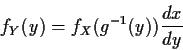
Step 1: Solve for x in terms of y: x=g-1(y).
Step 2: Remember the following basic equation
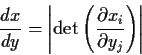
![\begin{displaymath}\left\vert\frac{dy}{dx}\right\vert =
\left\vert \mbox{det} \...
...rac{\partial y_p}{\partial x_p}
\end{array} \right]\right\vert
\end{displaymath}](img60.gif)
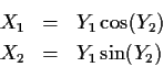
Example: The density
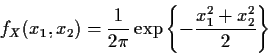
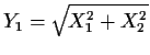 and Y2 is the angle (between 0 and
The first step is to solve for x in terms of y which gives
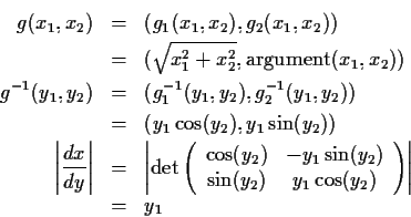
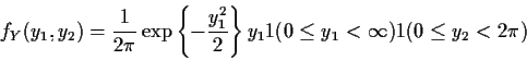
Next problem: what are the marginal densities of Y1 and Y2?
Note that fY can be factored into
fY(y1,y2) = h1(y1)h2(y2) where
It is then easy to see that
Note: When a joint density factors into a product you will always see the phenomenon above -- the factor involving the variable not be integrated out will come out of the integral and so the marginal density will be a multiple of the factor in question. We will see shortly that this happens when and only when the two parts of random vector are independent.
In the examples so far the density for X has been specified explicitly. In many situations, however, the process of modelling the data leads to a specification in terms of marginal and conditional distributions.
Definition: Events A and B are independent if
Definition: Events Ai,
![]() are
independent if
are
independent if
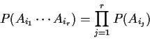
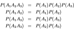
Example: p=3
Definition: Random variables X and Y are
independent if
Definition: Random variables
![]() are
independent if
are
independent if