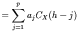
Postscript version of these notes
STAT 804: Notes on Lecture 5
Model identification
By model identification for a time series  we mean the process of selecting
values of
we mean the process of selecting
values of  so that the
 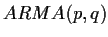 process gives a reasonable
fit to our data. The most important model identification tool is
a plot of (an estimate of) the autocorrelation function of ; we
use the abbreviation ACF for this function.
Before we discuss doing this with real data we explore what plots
of the ACF of various plots should look like (in the
absence of estimation error).
process gives a reasonable
fit to our data. The most important model identification tool is
a plot of (an estimate of) the autocorrelation function of ; we
use the abbreviation ACF for this function.
Before we discuss doing this with real data we explore what plots
of the ACF of various plots should look like (in the
absence of estimation error).
For an  process we found that
This has the important qualitative feature that it vanishes
for  .
.
For an  process
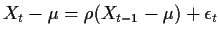 the autocorrelation function is
which has the qualitative feature of decreasing geometrically.
To derive the autocovariance for a general  we mimic
the technique for
we mimic
the technique for  . If
. If
 then
then
for  . Take these equations and divide through by
  and remember that
 and
and
 you see that the above recursions for
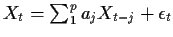
 are
are  linear
equations in the unknowns
linear
equations in the unknowns
 . They are
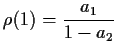
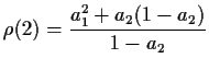
called the Yule Walker equations. For instance, when
. They are
called the Yule Walker equations. For instance, when  we get
which becomes, after division by
It is possible to use generating functions to get explicit formulas for
the  but here we simply observe that we have two equations in
two unknowns to solve. The second equation shows that
which is not possible if
but here we simply observe that we have two equations in
two unknowns to solve. The second equation shows that
which is not possible if  (unless
  ) and not a correlation for some other
  pairs. The first equation then gives
Notice that the Yule Walker equations permit to be calculated
recursively from
pairs. The first equation then gives
Notice that the Yule Walker equations permit to be calculated
recursively from  and
and  for
for  .
.
Now look at  , the characteristic polynomial, when we have
where
 are the two roots. Multiplying out we find
that
are the two roots. Multiplying out we find
that
 so that either one of the two has modulus
more than 1 (and the root
so that either one of the two has modulus
more than 1 (and the root
 has modulus less than 1) or
both have modulus 1. The two roots may be seen to be real so they would
have to be
has modulus less than 1) or
both have modulus 1. The two roots may be seen to be real so they would
have to be  . Since
 (again from multiplying
it out and examining the coefficient of
(again from multiplying
it out and examining the coefficient of  ) we would then know .
In either case there is no stationary solution.
) we would then know .
In either case there is no stationary solution.
Qualitative features: It is possible to prove that the
solutions of these Yule-Walker equations decay to 0 at a geometric rate
meaning that they satisfy
 for some
 .
However, for general they are not too simple.
.
However, for general they are not too simple.
Periodic Processes
If  are iid
 then we saw
is a strictly stationary process with mean 0 and
autocorrelation
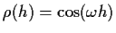 .
Thus the autocorrelation would be perfectly periodic.
.
Thus the autocorrelation would be perfectly periodic.
Linear Superposition
If and  are jointly stationary then
  is
stationary and
is
stationary and
Thus you could hope, for example, to recognize a periodic component
to a series by looking for a periodic component to a plotted
autocorrelation.
Periodic versus AR processes
In fact you can make AR processes which behave very much like
periodic processes. Consider the process
Here are graphs of trajectories and autocorrelations for
 and
and  .
.
 You should observe the slow decay
of the waves in the autocovariances, particularly for
You should observe the slow decay
of the waves in the autocovariances, particularly for  near 1.
When
near 1.
When  the characteristic polynomial is
  which has roots
Both these roots have modulus  so there is no stationary
trajectory with . The point is that some
so there is no stationary
trajectory with . The point is that some  processes have
nearly periodic components.
processes have
nearly periodic components.
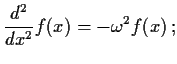
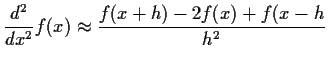
To get more insight consider the differential equation describing a
sine wave:
the solution if
 .
If we replace the derivative by differences we get the
approximation
so that
Take
.
If we replace the derivative by differences we get the
approximation
so that
Take  in the approximation and reorganize
to get
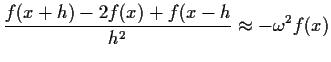
If we add noise, change notation to
in the approximation and reorganize
to get
If we add noise, change notation to  and replace the letter
 by we get
This is formalism only; there is no stationary solution of this
equation. However, we see that  processes are at least
analogous to the solutions of second order differential equations
with added noise.
processes are at least
analogous to the solutions of second order differential equations
with added noise.
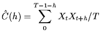
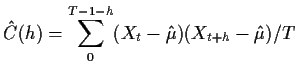
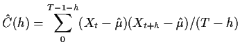
Estimates of  and
and 
In order to identify suitable  models using data we
need estimates of and . If we knew that
models using data we
need estimates of and . If we knew that  we would see that
We would then be motivated to use
simply averaging products over all pairs which are  time units
apart.
When
time units
apart.
When  is unknown we will often simply use
 and then
take
or, noting that there are only
and then
take
or, noting that there are only  terms in the sum
We then take
(Note, however, that when is used in the divisor it is technically
possible to get a
terms in the sum
We then take
(Note, however, that when is used in the divisor it is technically
possible to get a  value which exceeds 1.)
Richard Lockhart
2001-09-30
 Cov
Cov