Example 19.4: Linear Relations Among Factor Loadings

The CALIS Procedure

Example 19.4: Linear Relations Among Factor Loadings

The correlation matrix from Kinzer and Kinzer (N=326) is used by Guttman (1957) as an example that yields an approximate simplex. McDonald (1980) uses this data set as an example of factor analysis where he supposes that the loadings of the second factor are a linear function of the loadings on the first factor, for example

$b_{j2} = \alpha + \beta b_{j1} , j = 1, ... , n$

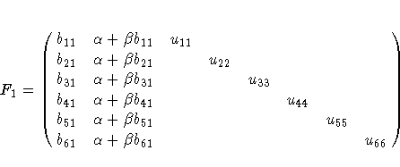
This example is also discussed in Browne (1982). The matrix specification of the model is

C = F₁F'₁

with

$F_1 = \pmatrix{b_{11}&\alpha + \beta b_{11}&u_{11}\cr b_{21}&\alpha + \beta b_{... ...beta b_{51}& & & & &u_{55}\cr b_{61}&\alpha + \beta b_{61}& & & & & &u_{66}\cr}$

This example is recomputed by PROC CALIS to illustrate a simple application of the COSAN model statement combined with program statements. This example also serves to illustrate the identification problem.

   data Kinzer(TYPE=CORR);                                      
   Title "Data Matrix of Kinzer & Kinzer, see GUTTMAN (1957)";  
      _TYPE_ = 'CORR'; INPUT _NAME_ $ Obs1-Obs6;                
      datalines;                                                
   Obs1  1.00   .     .     .     .     .                       
   Obs2   .51  1.00   .     .     .     .                       
   Obs3   .46   .51  1.00   .     .     .                       
   Obs4   .46   .47   .54  1.00   .     .                       
   Obs5   .40   .39   .49   .57  1.00   .                       
   Obs6   .33   .39   .47   .45   .56  1.00                     
   ;

In a first test run of PROC CALIS, the same model is used as reported in McDonald (1980). Using the Levenberg-Marquardt optimization algorithm, this example specifies maximum likelihood estimation in the following code:

   proc calis data=Kinzer method=max outram=ram nobs=326;         
      Title2 "Linearly Related Factor Analysis, (Mcdonald,1980)";   
      Title3 "Identification Problem";                              
      Cosan F(8,Gen) * I(8,Ide);                                   
      Matrix F                                                     
             [ ,1]= X1-X6,                                        
             [ ,2]= X7-X12,                                       
             [1,3]= X13-X18;                                      
      Parms Alfa = .5 Beta = -.5;                                   
         X7  = Alfa + Beta * X1;                                      
         X8  = Alfa + Beta * X2;                                      
         X9  = Alfa + Beta * X3;                                      
         X10 = Alfa + Beta * X4;                                      
         X11 = Alfa + Beta * X5;                                      
         X12 = Alfa + Beta * X6;                                      
      Bounds X13-X18 >= 0.;                                         
      Vnames F Fact1 Fact2 Uvar1-Uvar6;                             
   run;

The pattern of the initial values is displayed in vector and in matrix form. You should always read this output very carefully, particularly when you use your own programming statements to constrain the matrix elements. The vector form shows the mapping of the model parameters to indices of the vector X that is optimized. The matrix form indicates parameter elements that are constrained by program statements by indices of X in angle brackets ( < > ). An asterisk trailing the iteration number in the displayed optimization history of the Levenberg-Marquardt algorithm indicates that the optimization process encountered a singular Hessian matrix. When this happens, especially in the last iterations, the model may not be properly identified. The computed $\chi^2$ value of 10.337 for 7 degrees of freedom and the computed unique loadings agree with those reported by McDonald (1980), but the maximum likelihood estimates for the common factor loadings differ to some degree. The common factor loadings can be subjected to transformations that do not increase the value of the optimization criterion because the problem is not identified. An estimation problem that is not fully identified can lead to different solutions caused only by different initial values, different optimization techniques, or computers with different machine precision or floating-point arithmetic.

To overcome the identification problem in the first model, restart PROC CALIS with a simple modification to the model in which the former parameter X1 is fixed to 0. This leads to 8 instead of 7 degrees of freedom. The following code produces results that are partially displayed in Output 19.4.1.

   data ram2(TYPE=RAM); set ram;                                 
      if _type_ = 'ESTIM' then                                    
         if _name_ = 'X1' then do;                                 
            _name_ = ' '; _estim_ = 0.;                            
         end;                                                      
   run;                                                          
                                                                 
   proc calis data=Kinzer method=max inram=ram2 nobs=326;        
      Title2 "Linearly Related Factor Analysis, (Mcdonald,1980)";  
      Title3 "Identified Model";                                   
      Parms Alfa = .5 Beta = -.5;                                  
         X7  = Alfa;                                                 
         X8  = Alfa + Beta * X2;                                     
         X9  = Alfa + Beta * X3;                                     
         X10 = Alfa + Beta * X4;                                     
         X11 = Alfa + Beta * X5;                                     
         X12 = Alfa + Beta * X6;                                     
      Bounds X13-X18 >= 0.;                                        
   run;

Output 19.4.1: Linearly Related Factor Analysis: Identification Problem