MODEL Statement

The MIXED Procedure

MODEL Statement

MODEL dependent = < fixed-effects >< / options >;

The MODEL statement names a single dependent variable and the fixed effects, which determine the X matrix of the mixed model (see the "Parameterization of Mixed Models" section for details). The specification of effects is the same as in the GLM procedure; however, unlike PROC GLM, you do not specify random effects in the MODEL statement. The MODEL statement is required.

An intercept is included in the fixed-effects model by default. If no fixed effects are specified, only this intercept term is fit. The intercept can be removed by using the NOINT option.

You can specify the following options in the MODEL statement after a slash (/).

ALPHA=number

requests that a t-type confidence interval be constructed for each of the fixed-effects parameters with confidence level 1-number. The value of number must be between 0 and 1; the default is 0.05.

ALPHAP=number

requests that a t-type confidence interval be constructed for the predicted values with confidence level 1-number. The value of number must be between 0 and 1; the default is 0.05.

CHISQ

requests that $\chi^2$ -tests be performed for all specified effects in addition to the F-tests. Type III tests are the default; you can produce the Type I and Type II tests using the HTYPE= option.

CL

requests that t-type confidence limits be constructed for each of the fixed-effects parameter estimates. The confidence level is 0.95 by default; this can be changed with the ALPHA= option.

CONTAIN

has the same effect as the DDFM=CONTAIN option.

CORRB

produces the approximate correlation matrix of the fixed-effects parameter estimates. For ODS purposes, the label for this table is "CorrB."

COVB

produces the approximate variance-covariance matrix of the fixed-effects parameter estimates $\hat{{\beta}}$ . By default, this matrix equals $(X'\hat{V}^{-1}X)^{-}$ and results from sweeping $({Xy})'\hat{V}^{-1}({Xy})$ on all but its last pivot and removing the y border. The EMPIRICAL option in the PROC MIXED statement changes this matrix into "empirical sandwich" form. For ODS purposes, the label for this table is "CovB."

COVBI

produces the inverse of the approximate variance-covariance matrix of the fixed-effects parameter estimates. For ODS purposes, the label for this table is "InvCovB."

DDF=value-list

enables you to specify your own denominator degrees of freedom for the fixed effects. The value-list specification is a list of numbers or missing values (.) separated by commas. The degrees of freedom should be listed in the order in which the effects appear in the "Tests of Fixed Effects" table. If you want to retain the default degrees of freedom for a particular effect, use a missing value for its location in the list. For example,

   model Y = A B A*B / ddf=3,.,4.7;

assigns 3 denominator degrees of freedom to A and 4.7 to A*B, while those for B remain the same.

DDFM=CONTAIN

DDFM=BETWITHIN

DDFM=RESIDUAL

DDFM=SATTERTH

DDFM=KENWARDROGER

specifies the method for computing the denominator degrees of freedom for the tests of fixed effects resulting from the MODEL, CONTRAST, ESTIMATE, and LSMEANS statements.

The DDFM=CONTAIN option invokes the containment method to compute denominator degrees of freedom, and it is the default when you specify a RANDOM statement. The containment method is carried out as follows: Denote the fixed effect in question A, and search the RANDOM effect list for the effects that syntactically contain A. For example, the RANDOM effect B(A) contains A, but the RANDOM effect C does not, even if it has the same levels as B(A).

Among the RANDOM effects that contain A, compute their rank contribution to the (X Z) matrix. The DDF assigned to A is the smallest of these rank contributions. If no effects are found, the DDF for A is set equal to the residual degrees of freedom, N - rank(X Z). This choice of DDF matches the tests performed for balanced split-plot designs and should be adequate for moderately unbalanced designs.

Caution: If you have a Z matrix with a large number of columns, the overall memory requirements and the computing time after convergence can be substantial for the containment method. If it is too large, you may want to use the DDFM=BETWITHIN option.

The DDFM=BETWITHIN option is the default for REPEATED statement specifications (with no RANDOM statements). It is computed by dividing the residual degrees of freedom into between-subject and within-subject portions. PROC MIXED then checks whether a fixed effect changes within any subject. If so, it assigns within-subject degrees of freedom to the effect; otherwise, it assigns the between-subject degrees of freedom to the effect (refer to Schluchter and Elashoff 1990). If there are multiple within-subject effects containing classification variables, the within-subject degrees of freedom is partitioned into components corresponding to the subject-by-effect interactions.

One exception to the preceding method is the case when you have specified no RANDOM statements and a REPEATED statement with the TYPE=UN option. In this case, all effects are assigned the between-subject degrees of freedom to provide for better small-sample approximations to the relevant sampling distributions.

The DDFM=RESIDUAL option performs all tests using the residual degrees of freedom, n - rank(XZ), where n is the number of observations.

The DDFM=SATTERTH option performs a general Satterthwaite approximation for the denominator degrees of freedom, computed as follows. Let C = (X'V^-1X)^-, where ^- denotes a generalized inverse, and let $\theta$ be the vector of unknown parameters in V. Let $\hat{C}$ and $\hat{\theta}$ be the corresponding estimates.

We first consider the one-dimensional case, and consider l to be a vector defining an estimable linear combination of $\beta$ .The Satterthwaite degrees of freedom for the t-statistic

$t = \frac{\ell \hat{\beta}}{\sqrt{\ell \hat{C}\ell'}}$

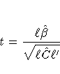
is computed as

$\nu = \frac{2 (\ell \hat{C} \ell')^2}{ g' A g}$

where g is the gradient of lC l' with respect to $\theta$ ,evaluated at $\hat{\theta}$ ,and A is the asymptotic variance-covariance matrix of $\hat{\theta}$ obtained from the second derivative matrix of the likelihood equations.

For the multi-dimensional case, let L be an estimable contrast matrix of rank q > 1. The Satterthwaite denominator degrees of freedom for the F-statistic

$F = \frac{ \hat{\beta}'L'(L\hat{C}L')^{-1} L \hat{\beta}}q$

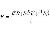
is computed by first performing the spectral decomposition $L\hat{C}L' = P' D P$ where P is an orthogonal matrix of eigenvectors and D is a diagonal matrix of eigenvalues, both of dimension q ×q. Define l_m to be the mth row of PL, and let

$\nu_m = \frac{2 (D_m)^2}{ g_m' A g_m}$

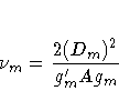
where D_m is the mth diagonal element of D and g_m is the gradient of l_m C l_m' with respect to $\theta$ ,evaluated at $\hat{\theta}$ . Then let

$E = \sum_{m=1}^q \frac{\nu_m}{\nu_m - 2}I(\nu_m \gt 2)$

where the indicator function eliminates terms for which $\nu_m \le 2$ .The degrees of freedom for F are then computed as

$\nu = \frac{2 E}{E - q}$

provided E > q; otherwise $\nu$ is set to zero.

This method is a generalization of the techniques described in Giesbrecht and Burns (1985), McLean and Sanders (1988), and Fai and Cornelius (1996). The method can also include estimated random effects. In this case, append $\hat{\gamma}$ to $\hat{\beta}$ and change $\hat{C}$ to be the inverse of the coefficient matrix in the mixed model equations. The calculations require extra memory to hold c matrices that are the size of the mixed model equations, where c is the number of covariance parameters. In the notation of Table 41.9, this is approximately 8q(p+g)(p+g)/2 bytes. Extra computing time is also required to process these matrices. The Satterthwaite method implemented here is intended to produce an accurate F-approximation; however, the results may differ from those produced by PROC GLM. Also, the small sample properties of this approximation have not been extensively investigated for the various models available with PROC MIXED.

The DDFM=KENWARDROGER option performs the degrees-of-freedom calculations detailed by Kenward and Roger (1997). This approximation involves inflating the estimated variance-covariance matrix of the fixed and random effects by the method proposed by Prasad and Rao (1990) and Harville and Jeske (1992); refer also to Kackar and Harville (1984). Satterthwaite-type degrees of freedom are then computed based on this adjustment. By default, the observed information matrix of the covariance parameter estimates is used in the calculations.

This method changes output in the following tables (listed in Table 41.7): Contrast, CorrB, CovB, Diffs, Estimates, InvCovB, LSMeans, MMEq, MMEqSol, Slices, SolutionF, SolutionR, Tests1 -Tests3. The OUTP= and OUTPM= data sets are also affected.

E

requests that Type I, Type II, and Type III L matrix coefficients be displayed for all specified effects. For ODS purposes, the labels of the tables are "Coefficients".

E1

requests that Type I L matrix coefficients be displayed for all specified effects. For ODS purposes, the label of this table is "Coefficients".

E2

requests that Type II L matrix coefficients be displayed for all specified effects. For ODS purposes, the label of this table is "Coefficients".

E3

requests that Type III L matrix coefficients be displayed for all specified effects. For ODS purposes, the label of this table is "Coefficients".

FULLX

requests that columns of the X matrix that consist entirely of zeros not be eliminated from X; they are eliminated by default. For a column corresponding to a missing cell to be added to X, its particular levels must be present in at least one observation in the analysis data set along with a missing dependent variable. The use of the FULLX option can impact coefficient specifications in the CONTRAST and ESTIMATE statements, as well as covariate coefficients from LSMEANS statements specified with the AT MEANS option.

HTYPE=value-list

indicates the type of hypothesis test to perform on the fixed effects. Valid entries for value are 1, 2, and 3; the default value is 3. You can specify several types by separating the values with a comma or a space. The ODS table names are "Tests1" for the Type 1 tests, "Tests2" for the Type 2 tests, and "Tests3" for Type 3 tests.

NOCONTAIN

has the same effect as the DDFM=RESIDUAL option.

NOINT

requests that no intercept be included in the model. An intercept is included by default.

NOTEST

specifies that no hypothesis tests be performed for the fixed effects.

OUTP=SAS-data-set

OUTPRED=SAS-data-set

specifies an output data set containing predicted values and related quantities. This option replaces the P option from Version 6.

Predicted values are formed by using the rows from (X Z) as L matrices. The predicted values from the original data are, thus, $X\hat{{\beta}} + Z\hat{{\gamma}}$ . Their approximate standard errors of prediction are formed from the quadratic form of L with $\hat{C}$ defined in the "Statistical Properties" section. The L95 and U95 variables provide a t-type confidence interval for the predicted values, and they correspond to the L95M and U95M variables from the GLM and REG procedures for fixed-effect models. The residuals are the observed minus the predicted values. Predicted values for data points other than those observed can be obtained by using missing dependent variables in your input data set.

Specifications that have a REPEATED statement with the SUBJECT= option and missing dependent variables compute predicted values using empirical best linear unbiased prediction (EBLUP). Using hats $(\hat{{}})$ to denote estimates, the EBLUP formula is

$\hat{m} = X_{m}\hat{{\beta}} + \hat{C}_{m} \hat{V}^{-1} (y- X\hat{{\beta}})$

where m represents a hypothetical realization of a missing data vector with associated design matrix X_m. The matrix C_m is the model-based covariance matrix between m and the observed data y, and other notation is as presented in the "Mixed Models Theory" section.

The estimated prediction variance is as follows:

$\hat{Var}(\hat{m} - m) &=& \hat{V}_{m}- \hat{C}_{m}\hat{V}^{-1} \hat{C}_{m}^T +... ...\hat{V}^{-1} X] ( X^T \hat{V}^{-1} X)^- [X_{m}- \hat{C}_{m}\hat{V}^{-1} X]^T$

where V_m is the model-based variance matrix of m. For further details, refer to Henderson (1984) and Harville (1990). This feature can be useful for forecasting time series or for computing spatial predictions.

By default, all variables from the input data set are included in the OUTP= data set. You can select a subset of these variables using the ID statement.

OUTPM=SAS-data-set

OUTPREDM=SAS-data-set

specifies an output data set containing predicted means and related quantities. This option replaces the PM option from Version 6.

The output data set is of the same form as that resulting from the OUTP= option, except that the predicted values do not incorporate the EBLUP values $Z\hat{{\gamma}}$ nor do they use the EBLUPs for specifications that have a REPEATED statement with the SUBJECT= option and missing dependent variables. The predicted values are formed as $X\hat{{\beta}}$ in the OUTPM= data set, and standard errors are quadratic forms in the approximate variance-covariance matrix of $\hat{{\beta}}$ as displayed by the COVB option.

By default, all variables from the input data set are included in the OUTPM= data set. You can select a subset of these variables using the ID statement.

SINGULAR=number

tunes the sensitivity in sweeping. If a diagonal pivot element is less than D*number as PROC MIXED sweeps a matrix, the associated column is declared to be linearly dependent upon previous columns, and the associated parameter is set to 0. The value D is the original diagonal element of the matrix. The default is 1E4 times the machine epsilon; this product is approximately 1E-12 on most computers.

SINGCHOL=number

tunes the sensitivity in computing Cholesky roots. If a diagonal pivot element is less than D*number as PROC MIXED performs the Cholesky decomposition on a matrix, the associated column is declared to be linearly dependent upon previous columns and is set to 0. The value D is the original diagonal element of the matrix. The default for number is 1E4 times the machine epsilon; this product is approximately 1E-12 on most computers.

SINGRES=number

sets the tolerance for which the residual variance is considered to be zero. The default is 1E4 times the machine epsilon; this product is approximately 1E-12 on most computers.

SOLUTION

S

requests that a solution for the fixed-effects parameters be produced. Using notation from the "Mixed Models Theory" section, the fixed-effects parameter estimates are $\hat{b}$ and their approximate standard errors are the square roots of the diagonal elements of $(X'\hat{V}^{-1}X)^{-}$ . You can output this approximate variance matrix with the COVB option or modify it with the EMPIRICAL option in the PROC MIXED statement.

Along with the estimates and their approximate standard errors, a t-statistic is computed as the estimate divided by its standard error. The degrees of freedom for this t-statistic matches the one appearing in the "Tests of Fixed Effects" table under the effect containing the parameter. The "Pr > |t|" column contains the two-tailed p-value corresponding to the t-statistic and associated degrees of freedom. You can use the CL option to request confidence intervals for all of the parameters; they are constructed around the estimate by using a radius of the standard error times a percentage point from the t-distribution.

XPVIX

is an alias for the COVBI option.

XPVIXI

is an alias for the COVB option.

ZETA=number

tunes the sensitivity in forming Type III functions. Any element in the estimable function basis with an absolute value less than number is set to 0. The default is 1E-8.

Chapter Contents
Previous
Next
Top