PROC MIXED Statement

PROC MIXED < options >;

makes the convergence criterion absolute. By default, it is relative (divided by the current objective function value). See the CONVF, CONVG, and CONVH options in this section for a description of various convergence criteria.

ALPHA=number

requests that confidence limits be constructed for the covariance parameter estimates with confidence level 1-number. The value of number must be between 0 and 1; the default is 0.05.

ASYCORR

produces the asymptotic correlation matrix of the covariance parameter estimates. It is computed from the corresponding asymptotic covariance matrix (see the description of the ASYCOV option, which follows). For ODS purposes, the label of the "Asymptotic Correlation" table is "AsyCorr."

ASYCOV

requests that the asymptotic covariance matrix of the covariance parameters be displayed. By default, this matrix is the observed inverse Fisher information matrix, which equals 2H^-1, where H is the Hessian (second derivative) matrix of the objective function. See the "Covariance Parameter Estimates" section for more information about this matrix. When you use the SCORING= option and PROC MIXED converges without stopping the scoring algorithm, PROC MIXED uses the expected Hessian matrix to compute the covariance matrix instead of the observed Hessian. For ODS purposes, the label of the "Asymptotic Covariance" table is "AsyCov."

CL<=WALD>

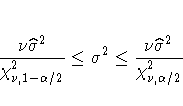
requests confidence limits for the covariance parameter estimates. A Satterthwaite approximation is used to construct limits for all parameters that have a default lower boundary constraint of zero. These limits take the form

$\frac{\nu \hat{\sigma}^2}{\chi^2_{\nu,1-\alpha/2}} \leq \sigma^2 \leq \frac{\nu \hat{\sigma}^2}{\chi^2_{\nu,\alpha/2}}$

where $\nu = 2Z^2$ , Z is the Wald statistic $\hat{\sigma}^2/{\rm se}(\hat{\sigma}^2)$ , and the denominators are quantiles of the $\chi^2$ -distribution with $\nu$ degrees of freedom. Refer to Milliken and Johnson (1992) and Burdick and Graybill (1992) for similar techniques.

For all other parameters, Wald Z-scores and normal quantiles are used to construct the limits. The optional =WALD specification requests Wald limits for all parameters.

The confidence limits are displayed as extra columns in the "Covariance Parameter Estimates" table. The confidence level is $1 - \alpha = 0.95$ by default; this can be changed with the ALPHA= option.

CONVF<=number>

requests the relative function convergence criterion with tolerance number. The relative function convergence criterion is

$\frac{| f_k - f_{k-1}|}{| f_k|} \leq number$

where f_k is the value of the objective function at iteration k. To prevent the division by |f_k|, use the ABSOLUTE option. The default convergence criterion is CONVH, and the default tolerance is 1E-8.

CONVG <=number>

requests the relative gradient convergence criterion with tolerance number. The relative gradient convergence criterion is

$\frac{{\rm max}_j | g_{jk}|}{| f_k|} \leq number$

where f_k is the value of the objective function, and g_jk is the jth element of the gradient (first derivative) of the objective function, both at iteration k. To prevent division by |f_k|, use the ABSOLUTE option. The default convergence criterion is CONVH, and the default tolerance is 1E-8.

CONVH<=number>

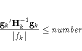
requests the relative Hessian convergence criterion with tolerance number. The relative Hessian convergence criterion is

$\frac{{g_k}' H^{-1}_k{g_k}}{| f_k|} \leq number$

where f_k is the value of the objective function, g_k is the gradient (first derivative) of the objective function, and H_k is the Hessian (second derivative) of the objective function, all at iteration k.

If H_k is singular, then PROC MIXED uses the following relative criterion:

$\frac{g_k'g_k}{| f_k|} \leq number$

To prevent the division by |f_k|, use the ABSOLUTE option. The default convergence criterion is CONVH, and the default tolerance is 1E-8.

COVTEST

produces asymptotic standard errors and Wald Z-tests for the covariance parameter estimates.

DATA=SAS-data-set

names the SAS data set to be used by PROC MIXED. The default is the most recently created data set.

DFBW

has the same effect as the DDFM=BW option in the MODEL statement.

EMPIRICAL

computes the estimated variance-covariance matrix of the fixed-effects parameters by using the asymptotically consistent estimator described in Huber (1967), White (1980), Liang and Zeger (1986), and Diggle, Liang, and Zeger (1994). This estimator is commonly referred to as the "sandwich" estimator, and it is computed as follows:

$(X'\hat{V}^{-1}X)^- (\sum_{i=1}^S X_i'\hat{V_i}^{-1} \hat{{\epsilon}_i} \hat{{\epsilon}_i}' \hat{V_i}^{-1}X_i ) (X'\hat{V}^{-1}X)^-$

Here, $\hat{{\epsilon}_i} = y_i - X_i\hat{{\beta}}$ , S is the number of subjects, and matrices with an i subscript are those for the ith subject. You must include the SUBJECT= option in either a RANDOM or REPEATED statement for this option to take effect.

When you specify the EMPIRICAL option, PROC MIXED adjusts all standard errors and test statistics involving the fixed-effects parameters. This changes output in the following tables (listed in Table 41.7): Contrast, CorrB, CovB, Diffs, Estimates, InvCovB, LSMeans, MMEq, MMEqSol, Slices, SolutionF, Tests1 -Tests3. The OUTP= and OUTPM= data sets are also affected. Finally, the Satterthwaite and Kenward-Roger degrees of freedom methods are not available if you specify EMPIRICAL.

displays a table of various information criteria. Four different criteria are computed in four different ways, producing 16 values in all. Table 41.2 displays the four criteria in both larger-is-better and smaller-is-better forms.

Table 41.2: Information Criteria

Criteria	Larger-is-better	Smaller-is-better	Reference
AIC	l- d	-2l+ 2d	Akaike (1974)
HQIC	l- d loglogn	-2l+ 2d loglogn	Hannan and Quinn (1979)
BIC	l- d/2 logn	-2l+ d logn	Schwarz (1978)
CAIC	l- d(logn + 1)/2	-2l+ d(logn + 1)	Bozdogan (1987)

Here l denotes the maximum value of the (possibly restricted) log likelihood, d the dimension of the model, and n the number of effective observations. In Version 6 of SAS/STAT software, n equals the number of valid observations for maximum likelihood estimation and n-p for restricted maximum likelihood estimation, where p equals the rank of X. In later versions, n equals the number of effective subjects as displayed in the "Dimensions" table, unless this value equals 1, in which case n reverts to the Version 6 values.

PROC MIXED evaluates the criteria for both forms using d equal to both q and q+p, where q is the effective number of estimated covariance parameters. In Version 6, when a parameter estimate lies on a boundary constraint, then it is still included in the calculation of d, but in later versions it is not. The most common example of this behavior is when a variance component is estimated to equal zero.

For ODS purposes, the name of the "Information Criteria" table is "InfoCrit."

INFO

is a default option. The creation of the "Model Information" and "Dimensions" tables can be suppressed using the NOINFO option.

Note that, in Version 6, this option displays the "Model Information" and "Dimensions" tables.

ITDETAILS

displays the parameter values at each iteration and enables the writing of notes to the SAS log pertaining to "infinite likelihood" and "singularities" during Newton-Raphson iterations.

LOGNOTE

writes periodic notes to the log describing the current status of computations. It is designed for use with analyses requiring extensive CPU resources.

MAXFUNC=number

specifies the maximum number of likelihood evaluations in the optimization process. The default is 150.

MAXITER=number

specifies the maximum number of iterations. The default is 50.

METHOD=REML

METHOD=ML

METHOD=MIVQUE0

METHOD=TYPE1

METHOD=TYPE2

METHOD=TYPE3

specifies the estimation method for the covariance parameters. The REML specification performs residual (restricted) maximum likelihood, and it is the default method. The ML specification performs maximum likelihood, and the MIVQUE0 specification performs minimum variance quadratic unbiased estimation of the covariance parameters.

The METHOD=TYPEn specifications apply only to variance component models with no SUBJECT= effects and no REPEATED statement. An analysis of variance table is included in the output, and the expected mean squares are used to estimate the variance components (refer to Chapter 30, "The GLM Procedure," for further explanation). The resulting method-of-moment variance component estimates are used in subsequent calculations, including standard errors computed from ESTIMATE and LSMEANS statements. For ODS purposes, the new table names are "Type1," "Type2," and "Type3," respectively.

MMEQ

requests that coefficients of the mixed model equations be displayed. These are

$[{X'\hat{R}}^{-1}X& {X'\hat{R}}^{-1}Z\* {Z'\hat{R}}^{-1}X& {Z'\hat{R}}^{-1} {Z + \hat{G}}^{-1} ] , [{X'\hat{R}}^{-1}y\ {Z'\hat{R}}^{-1}y ]$

assuming that $\hat{G}$ is nonsingular. If $\hat{G}$ is singular, PROC MIXED produces the following coefficients

$[{X'\hat{R}}^{-1}X& {X'\hat{R}}^{-1}{Z \hat{G}}\* {\hat{G} Z'\hat{R}}^{-1}X & ... ...{Z \hat{G} + \hat{G} } ] , [{X'\hat{R}}^{-1}y\ {\hat{G} Z'\hat{R}}^{-1}y ]$

See the "Estimating and in the Mixed Model" section for further information on these equations.

MMEQSOL

requests that a solution to the mixed model equations be produced, as well as the inverted coefficients matrix. Formulas for these equations are provided in the preceding description of the MMEQ option.

When $\hat{G}$ is singular, $\hat{{\tau}}$ and a generalized inverse of the left-hand-side coefficient matrix are transformed using $\hat{G}$ to produce $\hat{{\gamma}}$ and $\hat{C}$ , respectively, where $\hat{C}$ is a generalized inverse of the left-hand-side coefficient matrix of the original equations.

NAMELEN<=number>

specifies the length to which long effect names are shortened. The default and minimum value is 20.

NOBOUND

has the same effect as the NOBOUND option in the PARMS statement.

NOCLPRINT<=number>

suppresses the display of the "Class Level Information" table if you do not specify number. If you do specify number, only levels with totals that are less than number are listed in the table.

NOINFO

suppresses the display of the "Model Information" and "Dimensions" tables.

NOITPRINT

suppresses the display of the "Iteration History" table.

NOPROFILE

includes the residual variance as part of the Newton-Raphson iterations. This option applies only to models that have a residual variance parameter. By default, this parameter is profiled out of the likelihood calculations, except when you have specified the HOLD= or NOITER option in the PARMS statement.

ORD

displays ordinates of the relevant distribution in addition to p-values. The ordinate can be viewed as an approximate odds ratio of hypothesis probabilities.

ORDER=DATA

ORDER=FORMATTED

ORDER=FREQ

ORDER=INTERNAL

specifies the sorting order for the levels of all CLASS variables. This ordering determines which parameters in the model correspond to each level in the data, so the ORDER= option may be useful when you use CONTRAST or ESTIMATE statements.

The default is ORDER=FORMATTED, and its behavior has been modified for Version 8. Now, for numeric variables for which you have supplied no explicit format (that is, for which there is no corresponding FORMAT statement in the current PROC MIXED run or in the DATA step that created the data set), the levels are ordered by their internal (numeric) value. In releases previous to Version 8, numeric class levels with no explicit format were ordered by their BEST12. formatted values. In order to revert to the previous method you can specify this format explicitly for the CLASS variables. The change was implemented because the former default behavior for ORDER=FORMATTED often resulted in levels not being ordered numerically and required you to use an explicit format or ORDER=INTERNAL to get the more natural ordering.

The following table shows how PROC MIXED interprets values of the ORDER= option.

Value of ORDER=	Levels Sorted By
DATA	order of appearance in the input data set
FORMATTED	external formatted value, except for numeric
	variables with no explicit format, which are
	sorted by their unformatted (internal) value
FREQ	descending frequency count; levels with the
	most observations come first in the order
INTERNAL	unformatted value

For FORMATTED and INTERNAL, the sort order is machine dependent. For more information on sorting order, see the chapter on the SORT procedure in the SAS Procedures Guide and the discussion of BY-group processing in SAS Language Reference: Concepts.

RATIO

produces the ratio of the covariance parameter estimates to the estimate of the residual variance when the latter exists in the model.

RIDGE=number

specifies the starting value for the minimum ridge value used in the Newton-Raphson algorithm. The default is 0.3125.

SCORING<=number>

requests that Fisher scoring be used in association with the estimation method up to iteration number, which is 0 by default. When you use the SCORING= option and PROC MIXED converges without stopping the scoring algorithm, PROC MIXED uses the expected Hessian matrix to compute approximate standard errors for the covariance parameters instead of the observed Hessian. The output from the ASYCOV and ASYCORR options is similarly adjusted.

SIGITER

is an alias for the NOPROFILE option.

UPDATE

is an alias for the LOGNOTE option.