Chapter Contents
Previous
Next
|
Chapter Contents |
Previous |
Next |
| The PHREG Procedure |
PROC PHREG syntax is similar to that of the other regression procedures in the SAS System. For simple uses, only the PROC PHREG and MODEL statements are required.
Consider the following data from Kalbfleisch and Prentice (1980). Two groups of rats received different pretreatment regimes and then were exposed to a carcinogen. Investigators recorded the survival times of the rats from exposure to mortality from vaginal cancer. Four rats died of other causes, so their survival times are censored. Interest lies in whether the survival curves differ between the two groups.
The data set Rats contains the variable Days (the survival time in days), the variable Status (the censoring indicator variable: 0 if censored and 1 if not censored), and the variable Group (the pretreatment group indicator).
   data Rats;
      label Days  ='Days from Exposure to Death';
      input Days Status Group @@;
      datalines;
   143 1 0   164 1 0   188 1 0   188 1 0
   190 1 0   192 1 0   206 1 0   209 1 0
   213 1 0   216 1 0   220 1 0   227 1 0
   230 1 0   234 1 0   246 1 0   265 1 0
   304 1 0   216 0 0   244 0 0   142 1 1
   156 1 1   163 1 1   198 1 1   205 1 1
   232 1 1   232 1 1   233 1 1   233 1 1
   233 1 1   233 1 1   239 1 1   240 1 1
   261 1 1   280 1 1   280 1 1   296 1 1
   296 1 1   323 1 1   204 0 1   344 0 1
   ;
   run;
In the MODEL statement, the response variable, Days, is crossed with the censoring variable, Status, with the value that indicates censoring enclosed in parentheses (0). The values of Days are considered censored if the value of Status is 0; otherwise, they are considered event times.
   proc phreg data=Rats;
      model Days*Status(0)=Group;
   run;
Results of the PROC PHREG analysis appear in Figure 49.1.
Since Group takes only two values, the null hypothesis
for no difference between the two groups is identical to the
null hypothesis that the regression coefficient for
Group is 0. All three tests in the "Testing Global
Null Hypothesis: BETA=0" table (see the section "Testing the Global Null Hypothesis")
suggest that the survival curves for the two pretreatment
groups may not be the same.
In this model, the hazards ratio (or risk ratio)
for Group, defined as the exponentiation of the
regression coefficient for Group, is the ratio of the hazard
functions between the two groups.
The estimate is 0.551, implying that the hazard function for
Group=1 is smaller than that for Group=0. In
other words, rats in Group=1 lived longer than those
in Group=0.
In this example, the comparison of two survival curves is put in the form of a proportional hazards model. This approach is essentially the same as the log-rank (Mantel-Haenszel) test. In fact, if there are no ties in the survival times, the likelihood score test in the Cox regression analysis is identical to the log-rank test. The advantage of the Cox regression approach is the ability to adjust for the other variables by including them in the model. For example, the present model could be expanded by including a variable that contains the initial body weights of the rats.
Next, consider a simple test of the validity of the proportional
hazards assumption.
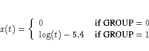
The proportional hazards model for comparing the two
pretreatment groups is given by the following:


   proc phreg data=Rats;
      model Days*Status(0)=Group X;
      X=Group*(log(Days) - 5.4);
   run;
|
| |||||||||||||||||||||||||||||
The analysis of the parameter estimates
is displayed in
Figure 49.2.
The Wald chi-squared statistic for
testing the null hypothesis that
![]() is 0.0158. The statistic is not statistically
significant when compared to a chi-squared distribution
with one degree of freedom (p=0.8999).
Thus, you can conclude that there is no
evidence of an increasing or
decreasing trend over time in the hazard ratio.
See the "Examples" section
for additional illustrations of PROC PHREG usage.
is 0.0158. The statistic is not statistically
significant when compared to a chi-squared distribution
with one degree of freedom (p=0.8999).
Thus, you can conclude that there is no
evidence of an increasing or
decreasing trend over time in the hazard ratio.
See the "Examples" section
for additional illustrations of PROC PHREG usage.
|
Chapter Contents |
Previous |
Next |
Top |
Copyright © 1999 by SAS Institute Inc., Cary, NC, USA. All rights reserved.