 |
VIBRATION |
Spectrum and Timbre
|
VIBRATION |
The classic (and highly simplified) distinction between acoustics and psychoacoustics is that the former deals with frequency, intensity and spectrum, where the latter involves their primary perceptual correlates, pitch, loudness and timbre, respectively. Perhaps this is a good start, but the first caveat is that each of these parameters is dependent on all the others. If we want to bridge the gap between lab experiments where variables are kept independently controllable (in both the fields of psychoacoustics and electroacoustic audio software) and aural perception in the everyday soundscape, we will need to understand how complex auditory input is processed as a whole during listening.
Of course, the scientific approach wants to bridge that gap too, by slowly and methodically building from basic processes to more complex ones. Fortunately, in recent decades, more cognitively based work has been done, but there are important clues to be learned here in this topic, and particularly in the subsequent module on Sound-Sound Interaction. We present four very broad categories here:(click on the link under the capital letter to go to that section)
A) Spectrum and its representations
B) Spectrum (or frequency content) and timbre (or tone colour) for sounds composed of discrete frequencies
C) Aperiodic vibration, continuous spectra and noise
D) Psychoacoustic phenomena
Q) Review quiz
home
A) Spectrum. The spectrum of a sound can be thought of as its frequency content. All sounds except for the sine wave consist of many individual frequencies and/or broadband components. Displays of these spectra tell us much more about the sound than, for instance, the waveform would. The basic problem for the representation of the spectrum is that it needs to be shown in three dimensions: frequency, amplitude or intensity, and time.
All forms of representation show what frequencies are present (preferably on a logarithmic scale that corresponds to how we hear – more on that a bit later) and with what strength, usually shown in decibels (dB). A two-dimensional representation of spectrum, where frequency is along the x-axis and amplitude is along the y-axis, parallels the conventional waveform diagram discussed in the first Vibration module.
Third-octave spectrum and sound of the Salvator Mundi bell
Here is a traditional 2-dimensional representation of a spectrum, that of a bell (the Salvator Mundi bell from Salzburg Cathedral). However, does it capture a moment in time – possibly misleading – or does it accumulate the maximum level achieved over its duration? This diagram is the latter, and was captured from a display (an analog instrument by Brüel & Kjaer) that operated in real-time, but allowed the max values to be accumulated (or not). Note the peak partials around 200, 315, 630 Hz, and the so-called “ring note”, much weaker at 80 Hz). This is not to say that there are no higher partials about 630 Hz, it’s just that they are too close together to be separately resolved by the 1/3 octave analysis. Technically these upper partials are called residue components.
The second point is: what is the bandwidth of the frequency analysis? In the Sound-Medium module under psychoacoustics, we noted that the ear’s discriminating sensitivity for spectrum (the critical bandwidth) was a little less than 1/4 of an octave, so the choice of this display as 1/3 octave is good in order to have some correspondence to aural perception. This spectrum analyzer then can be thought of as a set of filters, each tuned to the international 1/3 octave bands with 1 kHz as a reference, similar to the Graphic Equalizer model introduced in the Filter & Equalizer module where those bands could be controlled.
Thirdly, from the perspective of how we learn to understand visual displays of sound, is it intuitive to show frequency, low to high, from left to right, and amplitude on a vertical dimension? Well, both variables vie for the vertical dimension (low to high pitch, low to high amplitude). In this model, amplitude wins out, and we have to learn to interpret frequency as left to right.
Three-dimensional representations of Spectrum. There are two options for a spectral display to add the time dimension in real-time. The first is an automation of the above diagram which allows the maximum value to be shown along with the instantaneous spectrum, as shown in this video example of the same bell.
Compare this last frame of the video which shows the two-dimensional maximum spectrum (top green line) with a screenshot of the complete three-dimensional display shown and discussed below. Notice that many more partials are resolved in this display, presumably because more frequency bands are being analyzed. However, that is not to say that we would be able to discern them ourselves, as discussed below in the Psychoacoustics section.
A more detailed spectral analysis of the Salvator Mundi bell from the video (click to enlarge above image)
This second approach changes the dimensions of the display to what is arguably the most intuitive format, namely scrolling time from right to left leaving a temporal trace that can be read in the conventional manner of left to right; placing frequency on the vertical axis, low to high as they are referred to, and showing amplitude in darker lines on a black-and-model, or in increasingly bright colours in the contemporary examples of spectrograms as shown above and throughout the Tutorial.
Spectrogram of the Salvator Mundi bell (click to enlarge)
Historically, one of the first such analyzers, called a spectrograph (whose graphic output is a spectrogram or sonagram) dating from the 1940s, was used for analyzing speech with an electromechanical device that imprinted the output strengths of a range of frequencies as lighter and darker lines on a scrolled paper as shown below. The detail that was shown (known as "visible speech") can also be realized with today’s software that is specialized for speech acoustics, etc., for instance AudioSculpt.
Spectrograph (left) and a speech sonogram (right); source: Denes & Pinson
In this historical example, note the linear frequency scale at left which has the advantage of showing the higher range of frequencies where the auditory system is most sensitive (1-4 kHz), even as it confines the lower formants below 1 kHz into the bottom band. However, these upper “speech frequencies” were key to telephonic communication where the comprehension of speech was critical. By limiting the telephonic bandwidth from 300 Hz to 3 kHz, it allowed more efficient use of the telephone lines to multiplex multiple signals at the same time, an industrial process characterized by Jonathan Sterne in his book on the mp3 format as perceptual technics, and a forerunner of the mp3 data compression format.
Here is a video example of a spectrogram showing real-time spectral analysis on a logarithmic frequency scale. This example is of a nighttime soundscape in the Amazon as recorded by David Monacchi and is a good example of the Acoustic Niche Hypothesis of independent frequency bands for various species that will be discussed later.
Index
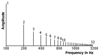
B) Spectra with discrete frequencies. The theoretical spectrum of a sound with discrete frequencies such as those in the Harmonic Series, shown already in the previous module, is called a line spectrum, and is a simple amplitude versus frequency diagram. It is "theoretical" because it does not come from a real-world analyzer which would have a limited resolving power to distinguish separate frequencies.
It is also quite distinct from a formant spectrum, e.g. for vowels, where the energy is concentrated in broader bands, or the continuous spectrum, where the energy is spread over a wide range of frequencies, as described below. Note that this line spectrum of a set of harmonics is shown on a logarithmic scale where octave doublings are equally spaced.
The harmonic series as a line spectrum
The typical line spectrum is based on the Fourier Theorem, which is a mathematical theorem stating that a periodic function f(x) which is reasonably continuous may be expressed as the sum of a series of sine or cosine terms (called the Fourier series), each of which has specific amplitude and phase, coefficients known as Fourier coefficients.
It was developed by the French mathematician Jean-Baptiste Joseph Fourier around 1800, as a general solution for polynomials, so it is unlikely he understood it in its acoustic context, since it was much later in the century that the German physicist Hermann von Helmholtz articulated it in acoustic terms in his famous book On the Sensations of Tone (1862).
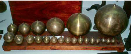
Helmholtz’s means of “analysis” was purely acoustic as well, based on a set of Helmholtz resonators each of which is a approximately spherical container with a small opening at one end and a larger one at the other, allowing it to be placed near the ear. The effect is similar to blowing across a bottle, but the spherical shape favours a single frequency which will be acoustically amplified, as described in the Sound-Medium Interface module. These resonators are more specifically tuned than the well-known effect of holding a conch shell to the ear and “hearing the sea”, which in fact (sorry to disrupt any illusions) is actually a resonator for the surrounding ambience.
A tuned set of Helmholtz resonators
The classic Helmholtz resonators were tuned to fixed frequencies, but a later development with two cylinders, one inside the other, could be tuned by sliding one of the cylinders to adjust the volume of air, and hence the pitch.
In this video example, we see and hear 14 harmonically related sine waves being added together to form a composite waveform. The oscilloscope at the left shows the waveform becoming increasingly complex as the harmonics are added, and the spectrogram at the right shows the spectral components being added one at a time. Note that the periodicity of the waveform – and hence its pitch – stays the same throughout. The amplitudes of the harmonics keep decreasing in strength, however the perceived timbre becomes richer, that is, more broadband in nature. The process is called additive synthesis, which is the opposite of the Fourier analysis.
As a footnote, the mathematical model requires a phase coefficient in order to be complete, but in this example, all the harmonics are in phase. If they were different, the resulting wave would look different, but sound approximately the same. Therefore, in practice the phase coefficient can be ignored unless it becomes variable or is modulated.
The limitations of the Fourier Theorem are also quite evident in this example. First of all, it can only result in a periodic waveform, which means it cannot be inharmonic. A simple way to understand this is that 2 periods of the 2nd harmonic, 3 of the 3rd, 4 of the 4th, and so on, add up to the same periodicity as the fundamental, the first harmonic – whereas that cannot happen when the individual periodicities are not integer multiples.
Secondly, and much more seriously, the timbre seem static and lifeless. Why? The third basic variable in a spectrum – time variation – is missing. In the early days of electronic music, the 1950s, Karlheinz Stockhausen became well known for his mixing of sine tone generators at the electronic music studio in Cologne, with equipment that had become available in broadcast studios after the World War. It is likely that he learned the Fourier approach from his mentor at the time Dr. Werner Meyer-Eppler.
These simple and monotonous sounds had not generally been heard before by musicians, and when combined, did not result in anything very aurally interesting (in a letter Stockhausen described them as “little brutes”). However, being an aurally sensitive composer, Stockhausen had the sense to feed his “tone mixtures” into the studio’s reverberation chamber which smoothed the timbre and made them more palatable, as can be heard in his famous Studie No. 1 and 2 from (1953-54).
This was an early example where a technological implementation based on an accepted theory or model exposed its shortcomings and led to improvements. Only a very few years later, the digital computer was able to participate in that process much more effectively.
Dynamic Spectra. The scene shifts to the Bell Telephone Laboratories, known as Bell Labs, in the U.S. and the pioneering work of Max Mathews and J. R. Pierce in digital sound synthesis. A French musician and scientist, Jean-Claude Risset, arrived there in the early 1960s with a desire to understand how musical timbre differed from the type of fixed waveform oscillator sound that lacked the complexity found in musical instruments.
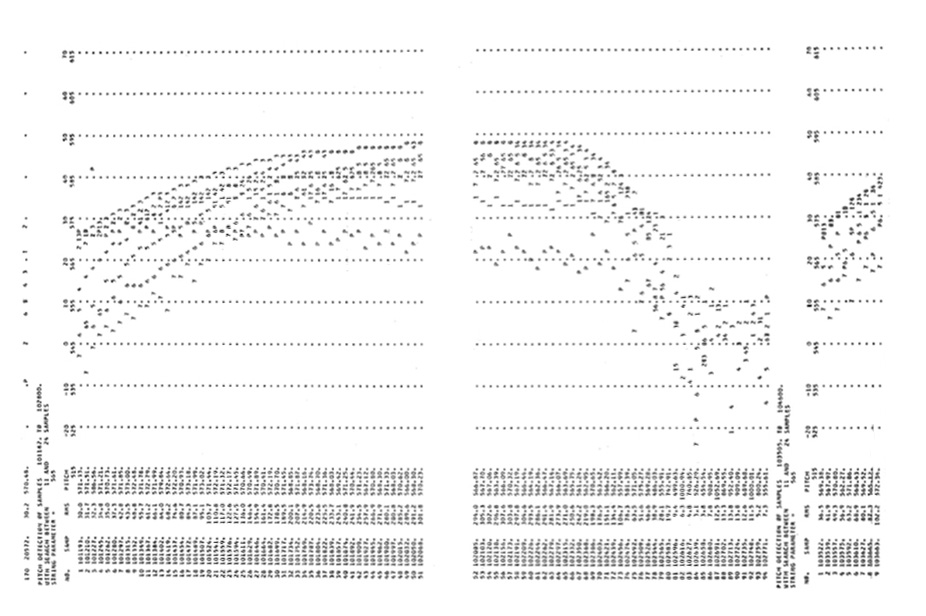
He proceeded by analyzing short instrumental tones with Fourier Analysis, but in this case, every period of the sound was digitally analyzed, a process called pitch synchronous analysis. A famous example from this work is the analysis of a very short trumpet tone (0.16 sec) with a fundamental frequency of 550 Hz (C sharp).
In this diagram, time, measured in units of single pitch periods, runs from right to left, because in practice there is no periodicity at the start of the sound, i.e. its attack. The transient nature of the attack is noisy (but highly important for the identification of instrument and how it was set into resonance), so periodicity could not be found. Instead, the analysis proceeded in the reverse direction from the end of the sound, and merely extrapolated the “periodicity” through the attack. It is also interesting to see the original data plot on which this diagram is based.
Spectral analysis of a brief trumpet tone by J. C. Risset at Bell Labs, in the 1960s
(click on diagram to see the original data plot)
The amplitudes of the first seven harmonics are shown in various graphic symbols, and reveal that they are never constant, even in the so-called “steady state” section of the tone in the middle. Also, at a more detailed level, the growth and decay of each harmonic doesn’t occur synchronously and the amplitude levels cross each other, meaning that there is no simple pattern related to harmonic number. True, the weaker, higher harmonics decay first, but even in such a short tone, the pattern is complex.
The result of this analysis shows that spectra are highly dynamic even in short sounds, and in fact, repetitions of the “same” note are going to be different. This raises the psychoacoustic question we will tackle below as to how the auditory system quickly identifies a sound with so much complexity, how it recognizes repetitions as being the same, and differentiates them from other simultaneous sounds.
Given this analysis, if we are going to implement a re-synthesis of the sound, it appears there is a great deal of data involved, so the next step would be to test a simplification of the amplitude envelopes by using linear breakpoints to describe them. However, this left the problem of the aperiodic attack transients. Data reduction in the amplitude envelopes, non-linear behaviour in the attack transients, and the non-intuitive control data (can you imagine specifying the envelope of the 3rd harmonic?) are and remain obstacles to the use of additive synthesis as a tool, despite its generality.
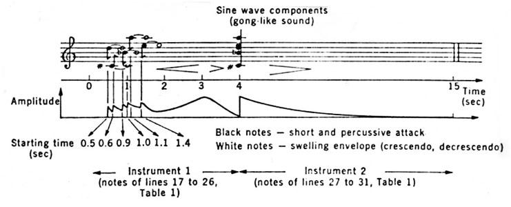
Before we proceed to the next research development, let’s look at how Risset switched roles from researcher to composer, using the Music IV and V languages that were created at Bell Labs. The first example (from Risset’s Catalogue) is a demonstration of pitch/timbre relationships. The frequencies in a gong-like sound are first heard separately, then fused into a complex sound. The fusion results because the attacks are now synchronous.
The second example is more compositional in that Risset starts with synchronous envelopes on a long series of arpeggiated bell-like sounds, then in two extensions, he de-synchronizes the envelopes, as shown at left, into beautiful waves of sound that become increasingly complex.
Adding partials together to synthesize a gong
Risset's additive gong
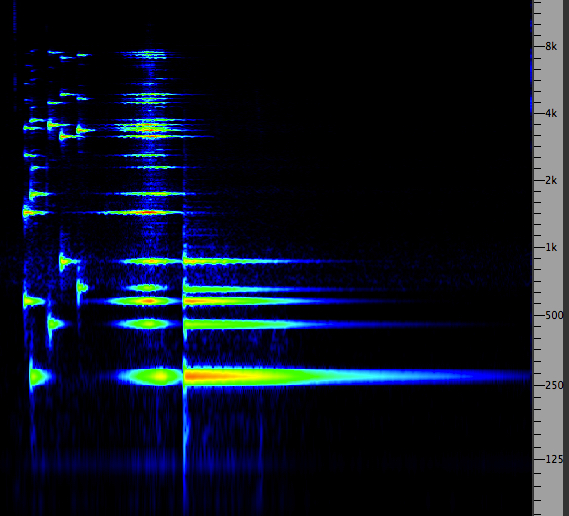
Risset's asynchronous envelopes (from Inharmonique)
as shown at left. and resulting spectrogram (below)
(click to enlarge)
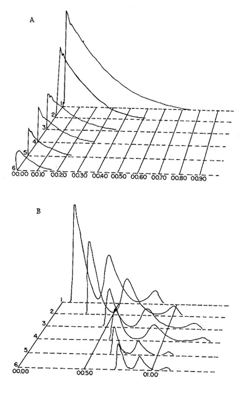
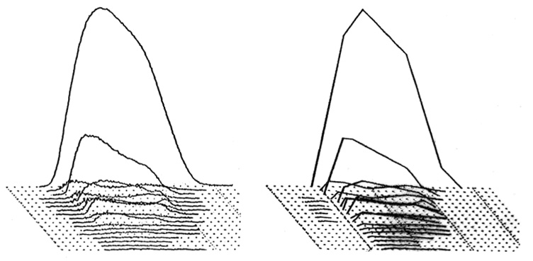
The scene now shifts to Stanford University and the CCRMA institute (pronounced “karma”). Composers John Chowning and David Wessel, along with their colleagues John Strawn and Andy Moorer, begin collaborating with the psychoacoustician John Grey on basically the same problem of musical timbre and its perception using digital analysis and synthesis. Here is one example of the data compression in additive re-synthesis mentioned above. In this representation, frequency is on the z-axis coming towards the front, with amplitude on the vertical.
Amplitude envelopes from the Fourier analysis of a clarinet tone (left) and their approximations (right)
The 3-dimensional spectral curves derived from Fourier Analysis for a clarinet tone are shown at the left, with their straight-line approximations at the right. Question: will they sound the same, or will some degradation be noticed by listeners? Answer is here.
To complete this brief survey of periodic spectra, a more significant result will be mentioned. Once we have the amplitude curves for each harmonic from a musical instrument, this data can be interpolated between different instruments, keeping the pitch the same. Timbre, that has often been regarded as discrete (similar to musical instruments themselves), could now be understood as occupying a continuum.
The following sound example is one of their demonstrations of a continuous trajectory. Since the sound quality is not the best, and the attacks are not well defined, here is how the trajectory is supposed to go:
clarinet ––> oboe ––> cello ––> horn ––> clarinet
To extend this approach, John Grey and his colleague John Gordon constructed a 3-dimensional timbre space model, based on extensive psychoacoustic testing with subjects who were asked to rate the distance (or similarity) between pairs of sounds. It is important to note that the subjects did not need to articulate how they sounded different, but rather to rate them on an arbitrary similar/dissimilar scale. The instruments shown below include French horn (FH), Cello (S), Flute (FL), Bassoon (BN), Trumpet (TP), Oboe (O), English horn (EH), Saxophone (X), Clarinet (C), and Trombone with mute (TM).
Through multi-dimensional scaling analysis, a number of dimensions can be uncovered to account for the subjective data. Then, by comparing this perceptual data to the acoustic analyses, the researchers were able to identify, in this case, three dimensions that seemed to be in play for timbre perception:
1) Spectral energy distribution (e.g. bright to mellow)Listening experiment. This examples has two versions, one that is a continuous trajectory in the timbre space, the other discontinuous, where some reverb is added to give a sense of an actual space. Which is the continuous one, A or B? Listen more than once preferably and try to imagine the sequence as connected. Answer here.
2) Attack synchronicity and fluctuation (often referred to as “bite”)
3) Attack spectrum (e.g. low amplitude, high-frequency energy in the attack, which is low for brass instruments and higher for strings)
Mapping of a timbre space by John Grey and John Gordon
The timbre space model has not become part of common practice, but it did achieve some significant results. It clearly demonstrated how multi-dimensional timbre perception is, and the methodology it used has been influential – starting with perceptual tests that by-passed the always tricky dependence on language about sound, and inferring its resulting models based on that data. The more traditional model, as we’ve outlined in the Sound-Medium Interface module, put the listener at the end of the chain of transfers, and has been dominated by the stimulus-response model in psychoacoustic research. Fortunately, a more listener centred model for soundscape perception is also starting to emerge.
Index
C. Aperiodic Spectra. One of many definitions of noise – the one that originated with Helmholtz – is that it is an aperiodic vibration that lacks pitch. Helmholtz preferred this objective, acoustic definition which worked well in terms of the Western ideal of music being pitched, while the noises of the street and factory were not. We will deal with definitions and measurement systems for noise in a later module, including attempts to quantify subjective responses as well as objective measurements.
In acoustic terms, the spectrum of an aperiodic vibration is continuous, as opposed to having discrete frequencies. There are few classifications beyond a simplistic one of referring to narrow-band noise, and broad-band, wide-band (or broadband) noise. Bandwidth is clearly a continuum, but some sounds like hiss are focused in a high-frequency octave. City ambience, heard at a distance, may be predominantly in the middle and low range, and some motors are mainly in the low frequency range.
Listen to the 6 sound examples under Broad-band Noise to get a range of typical spectra, both urban and natural. In terms of analysis involving broad-band sounds, the Fourier Theorem does not apply; instead, we use the generalized Fourier Transform which translates any sound from the time domain to the frequency domain. In practice, a more efficient version of the transform, namely the Fast Fourier Transform (FFT) is normally used, along with an inverse transform to go back to the time domain. The only problem with it in terms of perception is that it produces the analysis on a linear frequency scale, whereas the auditory system does its own analysis on a logarithmic scale. That means the FFT shows a lot of high frequency information that isn’t relevant for hearing.
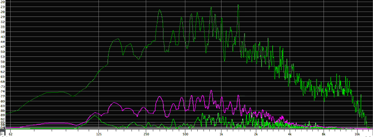
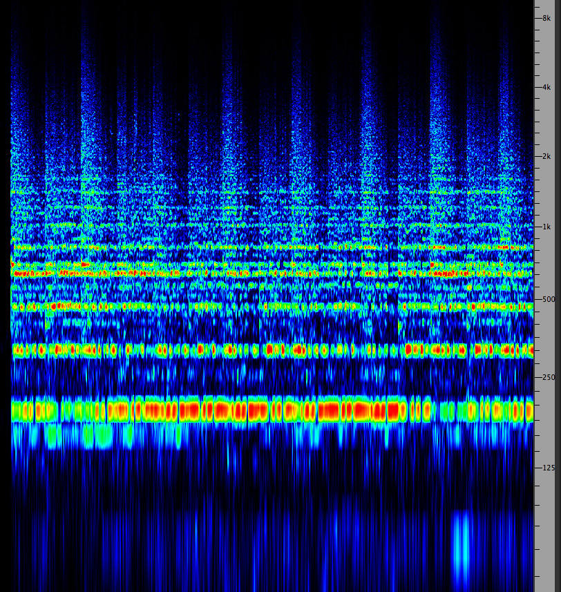
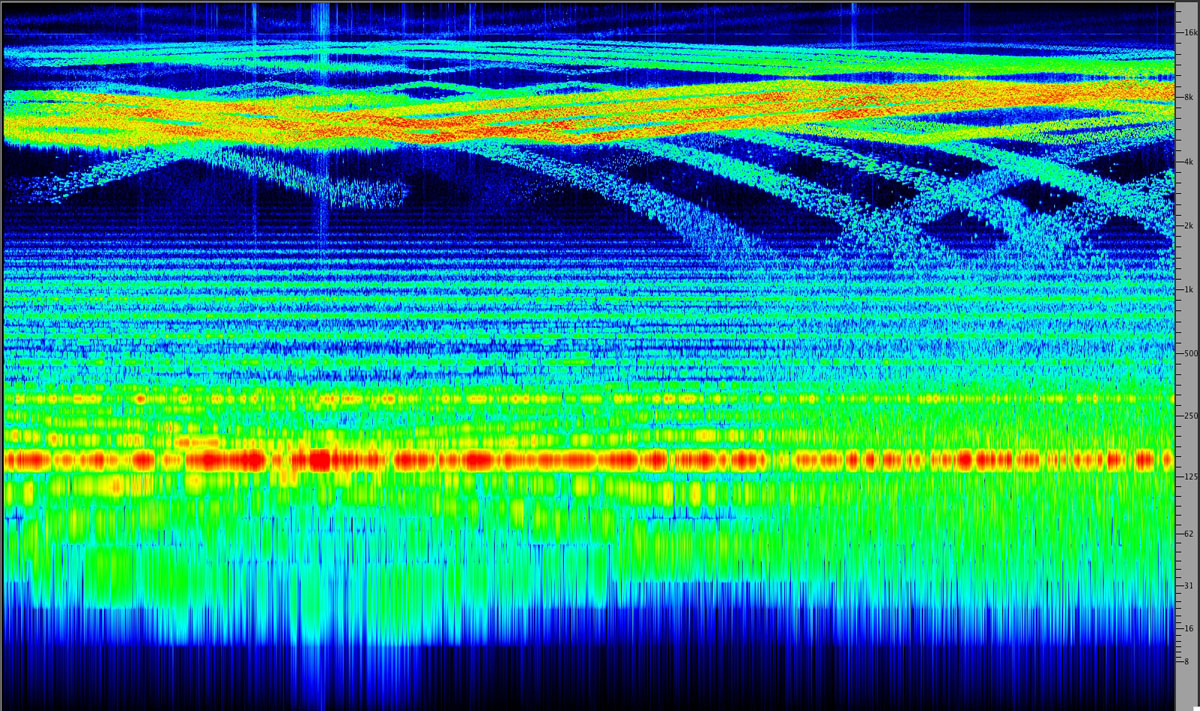
Left: Linear FFT analysis of section 5 of Riverrun (source: Helmuth);
Right: logarithmic spectrogram
Riverrun excerpt (Barry Truax)
What is remarkable is that, despite the ability of broadband sounds to cover up (i.e. mask) other sounds because of their large bandwidth, there are still instances where a pitched sound can “cut through” this wall of frequencies, mainly because of our sensitivity to pitch as covered in the previous module. All signals designed to attract attention are based on this principle.
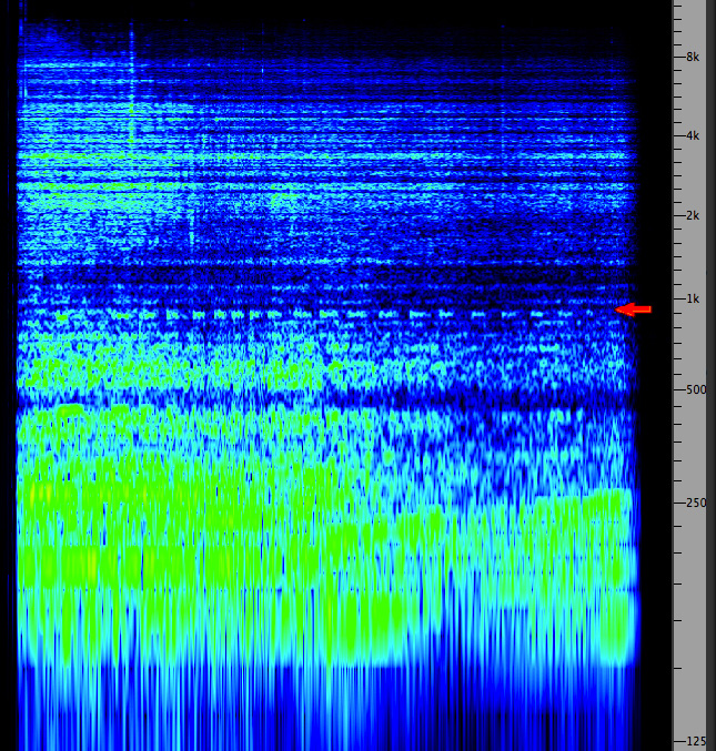
Take this example of a combine, for instance. You can focus on several components of the machine from the low to high frequency ranges, but still hear a pitched horn sounding simultaneously around 1 kHz in a small niche in the spectrum (marked with a red arrow). However this bit of periodicity cannot be seen in the waveform. What might look like quasi-periodicity is the low frequency throb of the motor.
Combine and horn
waveform and spectrogram
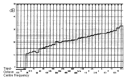
Synthetic noise can be created by a variety of both analog or digital means, and some can be classified according to their spectra. Two reference examples are called white noise and pink noise, although the colour analogies beyond “white” are tenuous. The white analogy is to white light that can be described as the composite of all colours equally, so therefore white noise is described as having all frequencies.
However, what is not often made clear is that “all frequencies” means on a linear scale, where 0 - 1 kHz has as much energy as 1 - 2 kHz, or 2 - 3 kHz. Since we hear on a logarithmic scale, a third-octave spectrum of white noise will show it weighted towards the high end, as shown below. And therefore, we find it extremely bright in timbre and texture, unpleasantly so, but if you adjust your volume as you listen, you can test that out. When used for test purposes (e.g. balancing speaker levels) white noise bursts are often used in order to add an attack and avoid aural adaptation.
Three bursts of white noise
and a typical third-octave spectrum analysis (right)
Keep in mind that low-level white noise has been installed in some open office spaces (at low levels) to supposedly mask unwanted sounds – except that pitched sounds can still cut through this imposed ambience, as you heard in the last (loud) sound example.
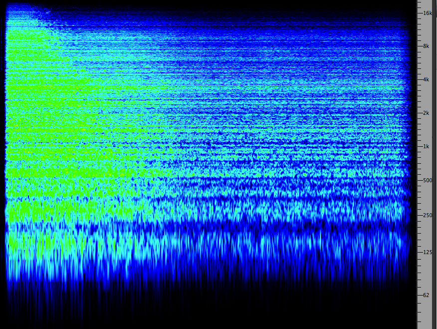
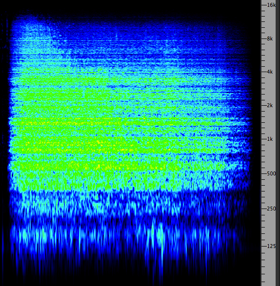
Pink noise, on the other hand is supposed to have equal energy in all octaves, so it should look flat on a log spectrum. It will also sound more pleasant (pinkish?), depending on the level.
Pink Noise
River
Interestingly enough, some naturally occurring broad-band sounds also have a fairly flat spectrum. Compare the pink noise to the river recording just below it. Both sounds have fairly consistent levels and spectra (note the yellow portions of the spectrogram). However, the river sound has a more interesting texture. Do you think that it is the textured quality of the sound, or the fact that you know it’s a river that makes you find it more pleasant? Or is it both?
The perception of aural texture is not as widely researched as is timbre in general. Short sounds that are iterated, i.e. repeated, closely together eventually create a texture (something halfway between the single and continuous energy input continuum shown in the Sound-Medium Interface module. Here are three sounds that have an interesting texture, or what is sometimes called grain, a term that was also used by Pierre Schaeffer in his list of qualities for the sound object (although he also included modulations such as vibrato and tremolo in the grain parameter).
The sounds are produced by (a) a güiro where a stick is drawn across the ribbed surface of a gourd, or wooden equivalent, open at one end, so the grains are fairly regular like a modulation; (b) a Chilean rainstick where a large number of cactus spines or pins are attached inside a hollow wooden tube which is filled with pebbles or other small objects that create a stochastic texture when the tube is angled; (c) carding wool by hand with a heavy brush with metal tines, which produces a constant broad-band texture. In fact, all of these sounds are broad-band in relatively narrow frequency ranges. Note how the envelope of each event of the güiro and carding indicate the manual gesture that was made to produce it.
The table allows you to hear these sounds at their original pitch, and then at 1, 2 and 3 octaves down, where the duration is doubled each time. These slower speeds allow you to hear micro patterns more easily (as well as any reverb in the original). How does the texture change? Some slower examples have been shortened (do you notice?).
Source
original pitch
-1 octave
-2 octaves
-3 octaves
Güiro
Rainstick
Carding
In conclusion, the perception of broad-band textured sounds needs further research. If we recall the three primary variables about spectrum (frequency, amplitude and time), and the historical progression we went through above, there was a certain point where the deficiencies of a fixed waveform model became apparent because there was no temporal component (e.g. the early electronic studio using sine waves or square waves). These studios usually had a noise generator as well which could be used with filters. This repertoire represented the sine wave at one end, and white noise at the other, as the continuum of sound spectra, even though they had few means to fill in what lay between.
To some extent, we are still at an analogous point with texture, although it is abundantly clear from the examples here that micro-time variations (which we generally do not see in the spectrogram displays) are quite clear when we listen to the sounds. There are some classifications such as a quasi-regular iteration of events, which moves towards modulation, or a stochastic distribution of events, which may be defined as a situation where we can perceive global properties such as density, tendencies or direction, and overall amplitude shapes, even though at the micro-level, sub-events are unpredictable. This latter experience occurs frequently in the acoustic environment with the sound of rain, for instance. We can say “it’s getting heavier or it’s letting up”.
What we are perceiving in these situations is what acousmatic musicians refer to as spectromorphology, the study of – quite literally – sound shapes. We will next turn to what we know about how the auditory system analyzes and decodes these shapes.
Index
D) Psychoacoustics. In this section we will cover four specific topics:
a) spectrum analysis in the inner ear(a) Based on what we saw above in terms of spectral analysis, we can start with a basic question:
b) pitch interaction with timbre
c) pitch paradoxes
d) temporal dependency of spectrum and timbre
Does the auditory system perform Fourier analysis?
The general answer is No. Before we go into the alternative, let’s consider some obvious problems if that were true:
- the huge amount of data involved in tracking N harmonics (how many would be necessary?) and their amplitudes, even with short soundsA slightly more nuanced answer to the question as to whether the auditory system can perform Fourier analysis, is that it has a very limited ability to do this under special circumstances. If you have a bit of time, you might like to try this experiment, similar to one conducted by the Dutch psychoacoustician Reiner Plomp in the 1960s, where subjects were asked to match a harmonic in a complex spectrum to one of two alternative sine tones.
- the next iteration of that same sound would produce different values
- if the same sound source could produce sounds in various pitch ranges, there would be little in common between these component sounds
- attack transients are not well suited for Fourier analysis and yet they identify the important information about what kind of energy began the vibration, the so-called excitation function
With a sustained sound, and some back-and forth repetition, it was possible to hear the harmonic that matched the complex tone, but only for lower harmonics where the spacing was greater than the critical bandwidth. Once you’ve tried doing this for awhile (and it does work), you’ll understand why Fourier analysis such as this is not an efficient way for the ear to process and identify timbres.
To understand how the auditory system does analyze spectra, we need to introduce a bit of the structure of the inner ear (and leave a lot of details to the Audiology module). The key component in the analysis is the behaviour of the basilar membrane inside the cochlea which activates groups of hair cells along its length, and then these hair cells fire impulses that are sent via the auditory nerve to the auditory cortex.
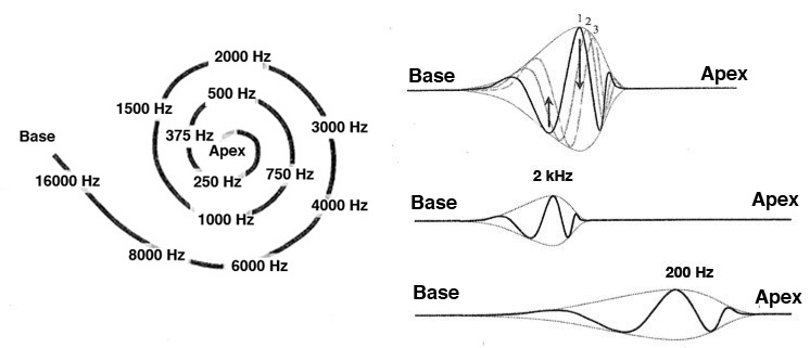
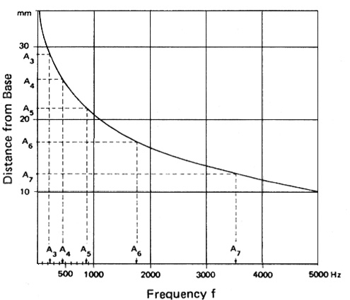
Using the 19th century model of Helmholtz resonators described above, it was initially thought that something similar was happening in the cochlea (basically the Fourier model). By the 1940s and later, a Hungarian biophysicist, Georg von Békésy, working in the US, showed that the range of audible frequencies was mapped onto the basilar membrane (coiled 2-1/2 times in the cochlea) with high frequencies stimulating the hair cells at the basal entrance to the cochlea, and low frequencies at the apical end. He received the Nobel prize for this work in 1961. These diagrams show a rolled and unrolled version of the basilar membrane related to the position of the resonant frequency in what is termed the place theory.
Frequency analysis along the length of the basilar membrane showing its logarithmic basis
All of these diagrams show the 35 mm length of the basilar membrane (which is amazing in itself as to how short this is - try spacing it on your hand to see how small this is). The upper right diagram also reminds us that there is a wave-like motion to these positions of resonance, not just a static “bulging” as it is sometimes referred to. The bottom diagram shows the basis of the logarithmic frequency distribution which has been mentioned several times already in the Tutorial.
The octaves of the pitch A are shown at left on the y-axis, mapped onto the 35 mm length, and on the x-axis, mapped onto frequency. These octave relations in frequency (i.e. doublings) are mapped onto equal distances along the membrane, hence the logarithmic nature of frequency analysis.
The main implication of this spatial mapping is that the cumulative resonance pattern along the membrane, in reaction to the entire spectrum, is a spatial one that is projected onto the auditory cortex retaining this spatial information. The pattern is what is usually called the spectral envelope, i.e. the pattern of resonances.
We have previously referred to the resolving power for frequency, which means, how far apart do the hair cells have to be to fire independently from the set on either side. In other words, what is the bandwidth of this analysis? The answer is the critical bandwidth, which is a little less than 1/4 octave, except below about 150 Hz. Approximately 24 critical bands cover the audible range. However, it should be kept in mind, this is not a “wiring diagram” – there are no fixed boundaries along this length; instead, the critical band is a relative distance, not an absolute one.
So, if you want to think about “data reduction” in the auditory system (compared with the massive amounts of data produced by Fourier analysis), here is the brilliant solution – processing in the inne ear turns the spectral analysis into a spatial pattern of about 24 points constituting a “shape” and combines it with a temporal envelope analysis for rapid recognition. This dual pattern of processing - relying on more than one type of analysis, in this case spatial and temporal – is typical of auditory functioning.
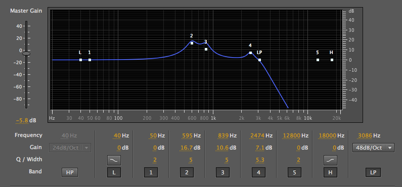
Filtered sawtooth wave, up and down,
followed by the same but with an EQ boost to simulate a vowel (which one?)
This example starts with a sawtooth wave that has been low-pass filtered to remove some the very annoying upper harmonics (the sawtooth wave has all the harmonics but they are very strong, with amplitudes that vary inversely with the harmonic number). It is then transposed up and down four semitones to show how the timbre changes slightly even in close ranges. Then you hear the same three transpositions with a fixed resonant boost with a parametric equalizer (see the link) designed to emulate (simplistically) the formants of a certain vowel.
This EQ, which changes the spectral envelope, stays fixed while the sawtooth wave goes up and down in pitch. Do you hear that something in the timbre now stays the same, independent of pitch (which is exactly what happens in speech where formants stay the same, with the same vocal tract resonance, while pitch inflections go up and down as the vocal folds vibrate faster or slower). Did you identify the vowel? (it’s the male “aw”).
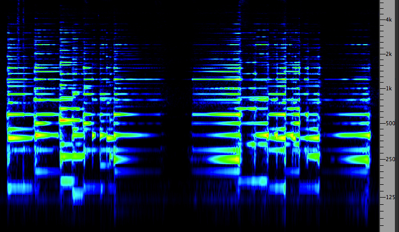
Next we hear a bassoon going up and down over a three octave range. Note how the timbre changes from the rich lower region to the thinner upper notes. In the next repetition, the top note is transposed to all of the other pitches in the scale, including the very lowest note. The timbre is seriously affected, particularly in the low register. This was a problem for early samplers that tried not to have a different sample for each pitch of a keyboard (not that playing a bassoon on a keyboard was such a great idea to start with!). Instrumental timbres are recognized to have a different "colour" in each of its registers, with lower notes being more richly coloured and higher notes purer.
This is why you can’t transpose speech, or musical pitches, more than a small interval apart without it sounding weird (like “chipmunk” speech with an upward transposed voice). The basic message for aural recognition is:
Formant regions in the spectral envelope are invariant and this assists recognition.
Bassoon scales, normal and transposed
Source: IPO 30
(click to enlarge)
Pitch interaction with Timbre. Up until this point, we have treated pitch and timbre as if they involved separate processes. Pitch is detected through the firing rate of the hair cells, with a very fine resolution; timbre perception is based on the spectral envelope shape along the basilar membrane, with a much coarser resolution. Of course, the last example with the bassoon showed that timbre typically changes with different pitch ranges, but do they influence each other in certain situations?
If you’d like try another psychoacoustic experiment involving sine tones, this one is much shorter and asks you to identify a pure octave (2:1 ratio) with sine tones. The result will show you that pure frequencies like this don’t produce the kind of octave relationships we are familiar with (or other intervals for that matter). They sound flat because our normal musical experience of such intervals is influenced by the timbres (and complex spectra) we are familiar with in musical instruments and that refine pitch perception.
Another instance of this kind of interaction that is experienced much more frequently is called the missing fundamental. Fourier analysis reveals that in a harmonic spectrum, the fundamental frequency called the 1st harmonic correlates to the pitch that is heard. In contrast, inharmonic spectra heard in various examples here in bells and carillons, do not have that property. A bell will be tuned to have a strike note that corresponds to its pitch (but is one of the component partials, not the lowest one), whereas the ring note, the one that usually lasts the longest, will be the lowest partial and is probably weaker than the strike note component.
The theory behind the missing fundamental is the same as with the Fourier Theorem, presented earlier. All of the various harmonics have the same cumulative periodicity as the fundamental. In other words, 2 periods of the 2nd harmonic, 3 of the 3rd, and so on, repeat at the same period as the fundamental. The video example at the start of this module showed the oscilloscope function that confirms this. As a result, the fundamental can be weak or missing, but the cumulative periodicity will still be the same. Here is a graphic to show this relationship.
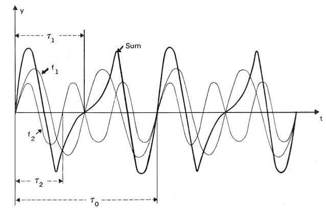
Addition of the second and third harmonics (light lines) to form a waveform (dark line) with the periodicity of the fundamental
In this diagram, we see the sum of the 2nd harmonic, labelled f1, and the 3rd harmonic, f2, along with their periods, as light lines. The dark line shows their sum and it can be seen that the second and third harmonics repeat at the same rate as the fundamental. Therefore since the auditory system is not analyzing harmonics separately, the periodicity in the composite waveform is that of the fundamental.
It is often noted that electroacoustic reproduction on speakers with limited bandwidth does not reproduce the fundamental frequency well. Examples are the small speakers or the telephone, where both the male and female voice are pitched below the normal bandwidth of the telephone which only transmits 300 Hz and above. The effect of this roll-off of the low frequencies on the phone is that the voice sounds more distant.
Early users of the phone – who typically shouted into it because they knew they were speaking across large distances – also recognized that the voice sounded distant as well. In addition, the psychological effect of having someone speaking directly into your ear at a very intimate distance could be normalized by allowing the voice to sound more distant than the actual location of the loudspeaker. The lower bandwidth (300 - 3 kHz) was sufficient to allow speech to be understood, to produce the illusion of a distant person, and to maximize profits by allowing more calls to travel on the same line.
Before we present a modern psychoacoustic demonstration of the missing fundamental, it would be interesting to listen to a short presentation of the topic that originated in the studio founded by Pierre Schaeffer in Paris, and was published in 1967. To complement Schaeffer’s large treatise on the sound object, the studio produced a tutorial type of recording called Solfège de l’objet sonore, with sound examples prepared by Guy Reibel and Beatriz Ferreyra to illustrate basic psychoacoustic phenomena that related to their work with real-world sounds.
Their approach was the opposite of the stimulus-response model of classic psychoacoustics that dominated work in North America at that time, and so the text often sounded a bit rebellious. But it also reflected their practical experimental work with recorded sound, known compositionally as musique concrète, as they isolated it in the studio and worked with its transformations. The original text was replaced with an English speaker at Simon Fraser University in this version.
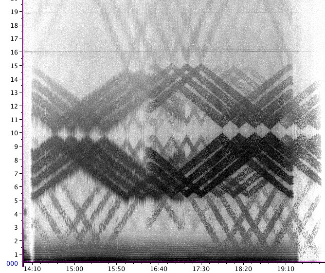
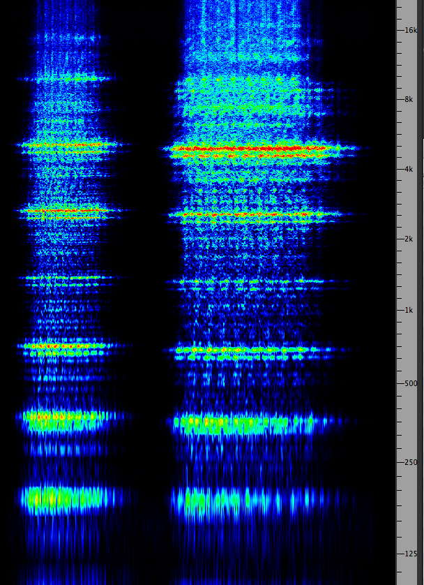
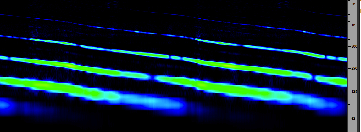
The missing fundamental, from the Solfège de l'objet sonore, 1967.
At right, the spectrogram of the transposed sound example near the end.
(click to enlarge)
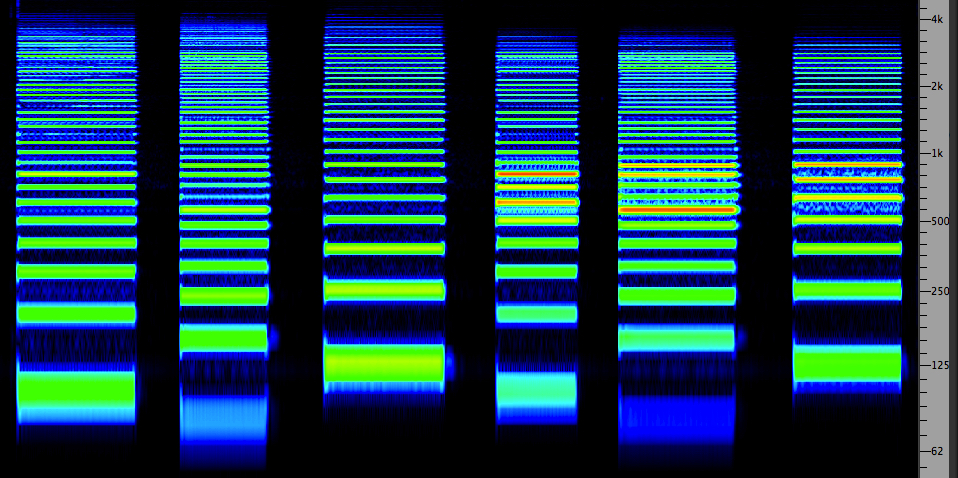
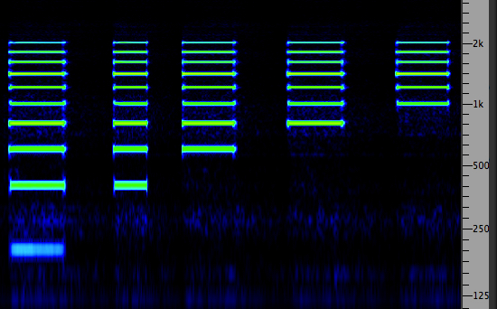
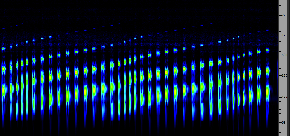
Progressive removal of harmonics
Source: IPO20
The example begins with 10 harmonics and a 200 Hz fundamental, then removes the 1st, 2nd, 3rd, 4th and 5th. Some low frequency noise is added to mask any difference tone. At first, the pitch stays the same, but once the 3rd harmonic is removed, it will appear to jump an octave (or more) since the periodicity now matches that of the second harmonic.
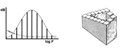
Pitch Paradoxes. Towards the end of the Schaeffer example above, a complex sound was played, then transposed down by playing it at half tape speed. Somewhat mysteriously, the pitch did not drop an octave, as expected, but only a semitone. A clue to the explanation lies in the spectrum as shown at the top right. It is primarily composed of strong octaves, so that when it’s transposed down an octave, other spectral pitches in the sound “replace” the original sense of pitch. It’s unclear as to why there’s a semitone change, but it’s possible that the upper octaves were slightly detuned.
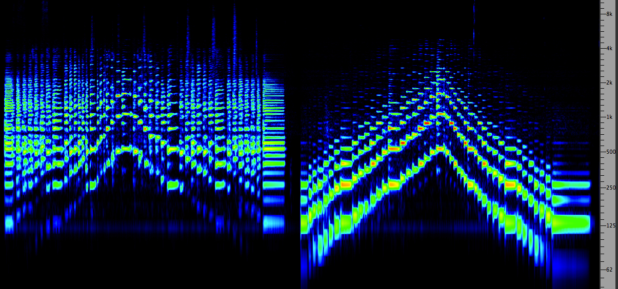
Shepard & Risset Pitch Paradoxes
(click to enlarge images)
Two other classic pitch paradoxes demonstrate the effect even more clearly. The first, created by Roger Shepard, and known as the “Shepard scale”, creates a circularity in discrete upward semitone steps. The signal is composed only of octaves that are passed through a fixed filter, the curved line shown at left. Since octaves fuse together, as the sequence moves up, lower octaves come in to replace the one determining the pitch, producing a seemingly endlessly ascending staircase, similar to the famous visual counterparts by M.C. Escher.
The second example, by Jean-Claude Risset, does something similar with a descending glissando. He also extended this demo example brilliantly in music that he composed for a play about the pilot of the Enola Gay, the plane that dropped the atomic bomb nicknamed Little Boy on Hiroshima. The music, which is part of Risset’s Computer Suite from Little Boy (1968), depicts not only the endlessly falling bomb, but the hallucination of the pilot as his mind descends into unreality.
In all of these examples, it is the spectral information that informs the perceived pitch progressions.
Temporal Dependency of Spectrum and Timbre. By “temporal dependency” we mean to focus on how the time domain affects timbral perception. The first examples put the emphasis on the attack transients at the beginning of a sound. They arrive first at the ear, and despite their brevity are the first bits of information that the auditory system receives to identify both the source of the sound and what kind of energy stimulated it into vibration. In fact, the recognition processes really goes in the opposite order:
what is the energy source and then what is the physical source being acted on.
Our first two sound examples illustrate this by reversing the sound, such that the attack is at the end, so we can hear what we are missing, so to speak. The first example is of a Bach chorale played on a piano, first in a forwards direction, and then with all of the piano notes played backwards (but with the pitches in the same order). Do you still hear a piano?
The second example plays 3 piano arpeggios in the low, middle and high ranges of the piano, each followed immediately by the reversed version of the arpeggio. How clearly can you heard the notes of the arpeggiated chords once they are reversed?
Bach chorale, forwards and reversed
Source: IPO29
(one phrase only)
Piano arpeggios, forwards and reversed
(click to enlarge images)
In the first example, the reversed sound of the piano is clearly not that of a piano, but something more like a “pump organ” with its characteristic wheezing sound as it pumps air through the pipes. The characteristic sharp attack of the piano is gone. Or you might have thought of an accordion activating its reeds with air.
In the second example, the arpeggiated notes are almost impossible to distinguish in the reversed versions, particularly in the low and high ranges, but a bit better in the middle one. Also notice with the reversed versions, how long the decay seems, now that it begins the sound; in fact, the forwards+reverse sequence doesn’t sound symmetrical at all. This phenomenon, related to precedence effect, will be discussed in the binaural localization module.
In this next example, the technique of cross-synthesis is used that combines the spectrum of one instrument with the temporal envelope of another, in order to show that for instrumental recognition, the temporal envelope is the stronger cue. First we have the piano spectrum with a flute envelope, followed by the flute itself, with each sound played twice. After a pause, we hear a flute spectrum with a piano envelope, following by the piano itself, also with each sound played twice.
Cross synthesis (a) flute spectrum with piano envelope, (b) piano spectrum with piano envelope
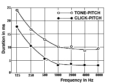
We now look at how the duration of a sound is perceived as a click when it is very short, from 4 - 10 ms depending on frequency, when pitch emerges with slightly longer durations, and then when a full tone with timbre can be determined. At the lower end of the scale, an uncertainty principle exists whereby the shorter the duration, the broader the bandwidth of the click. This will be discussed in more detail in the Microsound tutorial.
The following diagram shows the duration threshold below which sine tones lose their sense of pitch (upper curve) and become clicks (lower curve). Note that in the sound example, at 3 different frequencies, the number of periods is kept constant in each of the 8 repetitions. It is likely that you will start detecting pitch after the 4th repetition. Also note that our sense of pitch is much weaker at 3 kHz.
Tone sequences at 300 Hz, 1 and 3 kHz, lasting 1, 2, 4, 8, 16, 32, 64 and 128 periods
Source: IPO13
Then we turn to actual instrumental sounds by listening to increasing lengths of the sound and notice where a click becomes a pitch, then timbre emerges, and finally we hear the complete sound. The emergence of pitch comes first once the firing periodicity of the hair cells lasts long enough that its rate can be analyzed (after all, no repetitive pattern becomes clear until several cycles have elapsed). Given the fine resolution of pitch perception, this perception happens first.
Timbre perception, based on the spectral envelope, takes a little longer to process, and finally we hear the shape of the entire sound. Hence, the statement above that we identify the energy source first based on the attack, then the nature of the physical sound source itself, the timbre.
In the following examples, we include another historical segment from the Schaeffer Solfège where analog editing was used to isolate various segments of various instrumental sounds. The rest of the examples do something similar with digital editing on some Western and non-Western musical instruments.
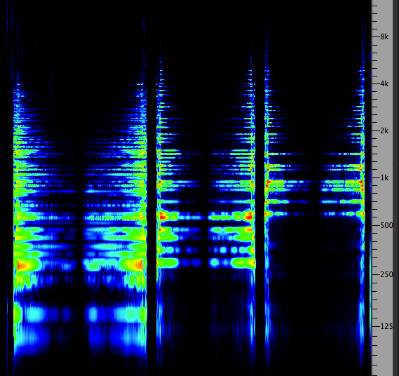
The time constants of the ear, from the Solfège de l'objet sonore, 1967.
Progressive segments of a Chinese zheng
attack noise, 3, 5, 10, 25, 50, 100, 250 ms
Same progression with a mid-pitched Indonesian gong
Same progression with a 12" tom
3, 7, 13, 25, 50, 100, 250 ms
Index
Q. Try this review quiz to test your comprehension of the above material, and perhaps to clarify some distinctions you may have missed. Note that a few of the questions may have "best" and "second best" answers to explain these distinctions.
home

