Most audio instructors and textbook authors would not expect
this topic to be introduced so early in the Tutorial, nor
would most of them consider pairing these two seemingly
unrelated topics. Ring modulation is a special case of modulation
in general (as introduced in the Electromagnetic section of
the Sound-Medium Interface module in the context of radio
transmission). It is often associated with the early
electronic music studios of the 1950s and 60s, where custom
hardware multiplied two signals (and hence was sometimes
called product modulation), with a typically noisy,
broadband result. Today it is not commonly found in the
contemporary digital world of plug-ins.
Auto-convolution is a special case of the general topic of Convolution which will be
presented in more detail in a later module. Briefly,
auto-convolution multiplies the spectrum of a sound with
itself, based on a non-real-time calculation involving
analysis with the FFT (Fast Fourier Transform). The length of
the sound is doubled, the spectrum thinned out to emphasize
its strongest components, and aurally, the result is usually
very attractive.
So, why present these two topics here, and why pair them up?
Well, let’s think outside the box. The answer to the first
question is that they both affect the frequency domain,
but unlike the filters and equalizers of the previous module
which worked linearly, these two methods work non-linearly.
By linear and non-linear, we are not referring to the linear
vs logarithmic distinction, usually applied to frequency.
Instead, a linear process means the output is proportional
to the input in some way. In the case of filters and
equalizers, nothing in the output spectrum in terms of
frequency is different from the input, just the relative
strengths of the parts of the spectrum being altered. In a non-linear
process, the output contains elements that are not
proportional to the original spectrum. For instance, new
frequency components will be present (as in ring modulation),
or a non-proportional filtering of the amplitudes of various
frequencies will occur, as in auto-convolution. To understand
what those new components are, you need to understand some
theory, as presented below.
In addition, at least two other characteristics of these two
processes link them together. They both require two input
signals and produce one output signal. As a
result they do not follow the standard format of a plug-in
which is one input, one output. In any implementation of these
processes, a second input will be required, so where does it
come from? This problem has possibly limited their
availability in a DAW.
Lastly – and most importantly – Ring Modulation and
Convolution in general are mathematically linked, as
diagrammed here in terms of the time domain (the waveform) and
the frequency domain (the spectrum):
TIME DOMAIN
<––––––––––> FREQUENCY DOMAIN
Convolution <––––––––––––> Multiplication
Multiplication <–––––––––> Convolution
This means
that when you convolve (note the verb, it’s not
“convolute” which means something else that we are trying to
avoid!) two signals in the time domain you multiply them in
the frequency domain, meaning you multiply their spectra.
And when you multiply them in the time domain, you are
convolving their spectra, and it’s called Ring Modulation!
We will now build up the necessary background to understand
these two processes in the following sections.
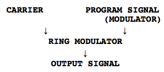
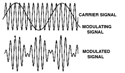
A. Modulation
is a process whereby the modulator or program signal
controls a parameter of the other signal, called the carrier.
In other words, the instantaneous value of, for instance,
the amplitude or frequency of the carrier takes on the
pattern of the modulator. The modulator’s waveform
information is thereby encoded into the carrier. The
result is a modulated
carrier.
All forms of modulation at audio rates (i.e. greater
than 20 Hz) produce added spectral components in the output
signal called sidebands. When the modulation is subaudio
(i.e. less than 20 Hz) audible changes in the carrier’s
parameter can be discerned. In the acoustic world, tremolo
refers to a rapid alteration of amplitude, for instance with
a vibraphone, whereas vibrato
refers to a rapid alteration of frequency, and hence pitch,
in the voice or a string instrument, for instance. Sometimes
these processes get confused, or even overlap.
The basic circuit for all modulators, including ring
modulation can be diagrammed as having two inputs and one
output. As noted above, this puts the process in an awkward position
to be implemented as a plug-in. The only attempt I’ve seen
is where the modulator is a built-in sine wave with a range
of about 0 - 300 Hz, which is not very generalized.
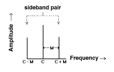
The three
types of modulation we are considering here result in
sidebands that can be predicted by a simple formula. Here we
assume that both input signals are sine waves, such as C
for the carrier and M for the modulator. The
sidebands then are also pure frequencies.
In the case of ring modulation, the two
signals are multiplied together, so there is no distinction
between carrier and modulator; therefore, we will refer to
them as X and Y. Sidebands always occur in pairs
that can be called upper and lower sidebands
as they are equally spaced around the carrier (if it is
present). Here is the general pattern.
TYPE of
MODULATION
SPECTRUM
Amplitude
C, C + M, C - M
Ring
X + Y and X - Y
Frequency
/ C ± n.M / for n =
0, 1, 2, 3, .... where n is the sideband
pair number
Amplitude
Modulation (AM), where the carrier’s amplitude
is determined by the waveform of the modulator, is similar
to Ring Modulation (RM) in the sense that multiplication of
two signals in RM is also affecting the output amplitude of
the waveform. The difference between them is that the carrier
frequency is present in the output spectrum of AM, but
is absent from the output spectrum of RM.
As we will see below, that means that RM can act as a pitch
shifter since neither input signal is present in the output
spectrum. Frequency
modulation (FM) produces a more complex spectrum
based on a
theoretically infinite set of sideband pairs,
equally spaced around the carrier. This will be discussed in
more detail below.
In all cases of modulation, the modulating frequency is
never present in the output spectrum, but instead, it
controls the spacing of the sidebands, hence the
density of the spectrum. The depth
of modulation in AM reflects the amplitude of
the modulator, and is usually controlled by a gain factor.
The stronger the amplitude of the modulator, the stronger
the sidebands.
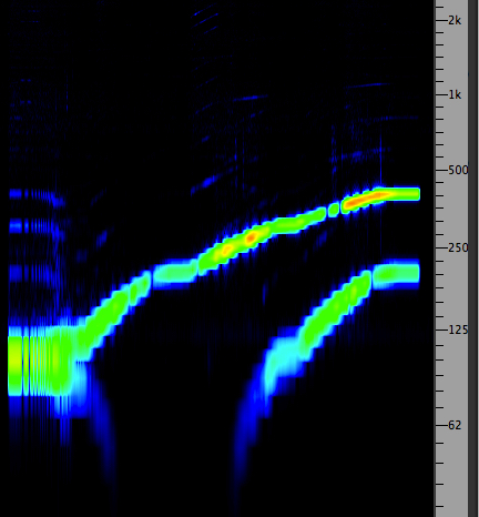
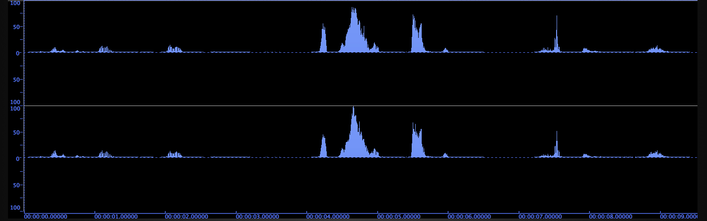
The following example
illustrates the typical type of spectrum produced by
Ring Modulation. There are only two sidebands,
which are the sum and difference (X + Y and X -
Y) and no carrier. In the example, we take a
constant 100 Hz signal as X, which is multiplied by a
signal Y that sweeps upwards from 0. The sum and
difference sidebands create a typical pattern of the sum
increasing and the difference falling, eventually
reaching zero when X and Y are identical. At that point
the sum is 2X, the octave above. Beyond that the
difference tone is reflected back into the
positive domain and starts ascending again. Eventually
both sum and difference tones lie high above the
original tone X.
Theoretically RM could be used for sound synthesis, but
it is not very general or flexible. For instance, there
will only be a harmonic relationship in the output if X
and Y are in a simple frequency ratio. All other cases
will be inharmonic and quite dissonant. Therefore in the
next section we look at RM as a non-linear signal
processor.
Ring modulating 100 Hz with an ascending
sine wave starting at zero
B. Ring Modulation (RM)
as a Processor. Using sine tones to learn about
RM is a good idea because we can hear the effects
quite clearly. However, once we depart from the pure
sine wave and start using more complex tones, not to
mention recorded samples, the output becomes noisy
very quickly because every frequency in the spectrum
gets doubled and hence the result is very dense.
However, using a complex sound as one input and a sine
wave as the second input, which we’ll call the
modulator, the result is often quite useful. There are
four general types of effects, depending on the
frequency range of the modulator in relationship to
the other sound.
MODULATOR RANGE
EFFECT
subaudio
range (< 20 Hz)
AM style
beating (or chopping if a square wave is
used)
same
range as carrier
added
spectral components
equal to
carrier
octave
pitch shift
much
higher than carrier
entire
signal shifted to high frequency
We’ll deal first with the “special case” of X and Y
(carrier and modulator) being identical. The
sum is 2X, the octave shift, and the
difference is zero, which is not a sound, but rather
can be described as a DC (Direct
Current) component. An audio signal alternates
positive and negative, whereas DC is a constant
voltage.
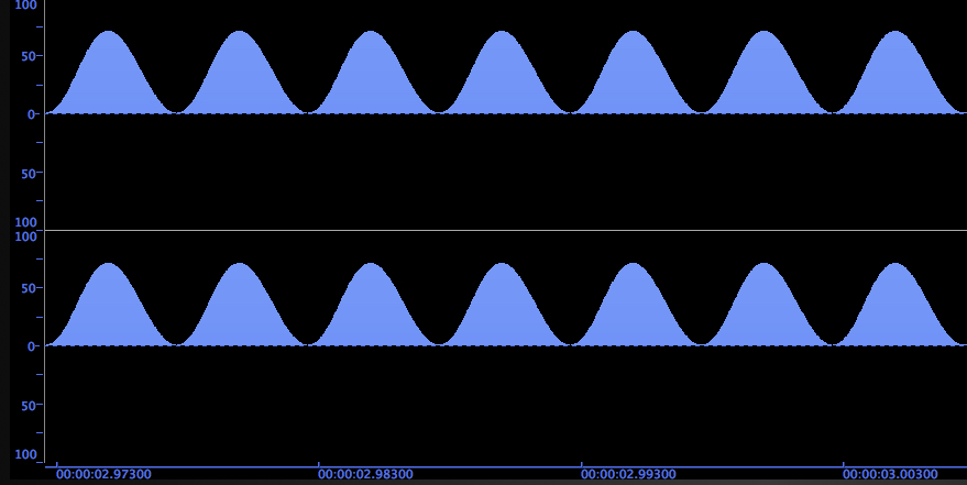
As you can see from the waveform diagrams below, that
raises a 100 Hz sine tone entirely into the positive
voltage domain and doubles the frequency. This effect
is also called a rectified
waveform, and the resulting DC component can become
undesirable in certain circumstances. In the case of
the sine wave, it just sounds thinner.
However, when we use a voice, for
instance, all of its frequencies are shifted up an
octave (including formant regions that are expected to
remain constant despite pitch shifts). However, it
does not sound like a doubling of pitch, the so-called
"chipmunk effect", because of phase differences that
are introduced, plus the DC component and the
non-linear loudness change with the louder phrases.
With the piano arpeggio, the normal pitch doubling
raises the sound by an octave as expected, but with a
brighter timbre. However, the self modulation example
almost seems to pitch the sound downward with a
striking timbral change. Since we’re talking about
auto-convolution below, this effect could be called
auto-ring modulation, but so far that term hasn’t
appeared generally.
SOURCE
ORIGINAL
OCTAVE
TRANSPOSITION
RM
with itself
WAVEFORM
Click to enlarge
Sine Wave
Voice
(Christopher Gaze)
Piano Arpeggio
Another special case is where there
is an octave relation between X and Y. The sum
and difference are 3X and X – the only case
where the original frequency appears in the output
spectrum, but only because the lower sideband matches
it. This effect is illustrated in the table below. The
waveform is no longer rectified and the original pitch
is restored but with an added 3rd harmonic.
Arguably the most useful range for RM is where you use
a sine tone in a similar range to your sound. The
examples show the effect with 100 Hz and 1 kHz
modulators modulating the voice and the piano
arpeggio. The effect is a classic non-linear
spectrum shift in that a constant frequency is
being added and subtracted from each spectral
component, thickening the timbre and adding dissonance
(unless a carefully tuned relationship with the
modulator has been arranged, such as the octave
examples).
SOURCE
RM
with Octave
RM
with 100 Hz
RM
with 1 kHz
Voice
Piano Arpeggio
Normal transpositions would use a constant ratio
(e.g. 2:1 or 3:2) because of the logarithmic nature of
hearing. Simply adding or subtracting a constant
amount will add many inharmonic partials not
in the original spectrum. GRM Tools has a Frequency
Shift module that is basically the upper
sideband of RM, the sum frequency, which is quite easy
to control.
The one caveat to using a sine wave soundfile for this
process is that it has to be at least as long as the
sound you want to process. Since you’re multiplying
the two signals, if one goes to zero (i.e. ends), then
nothing comes out – anything multiplied by zero is
zero.
The very high frequency modulator simply
shifts all frequencies to its high range. After all, 8
kHz plus or minus some lower frequencies still keeps
everything in the high range. This “disappearance” of
the input signal is possibly yet another reason for
the lack of popularity of RM in conventional signal
processing, where a purely linear process will colour
the input, but not make it disappear! Back in the
analog studio days, if someone wanted a “space alien
voice”, this is exactly what came to mind - high
frequency RM. How many sci-fi movies exploited that
one!
Voice with 8 kHz RM
The subaudio modulator goes
back to a straightforward multiplication of the
carrier signal with the slow pulse of whatever
waveform is used. If it’s a subaudio sine wave, then a
gentle tremolo is added, but if it’s a square
wave, the result chops up the signal with a
kind of pulsating stutter.
SOURCE
RM
with 6 Hz Sine Wave
RM
with 6 Hz Square Wave
Voice
Piano Arpeggio
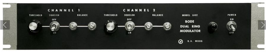
One
of the most famous Ring Modulators was designed by the
Norwegian engineer Harald Bode for Robert Moog. It had
two channels with two inputs each and a threshold
level control in order to minimize the “leakage”
of the input signal into the output. That is, any DC
offset in the audio signal going in (i.e. any
departure from equal positive and negative parts of
the signal) would act like a constant and also be
multiplied by the modulator signal which would cause
it to be heard in the background. Digital signals may
be less likely to have this DC component, but the same
effect will be heard if they do.
Classic analog Ring Modulator designed by Harald
Bode for Robert Moog
One
speculation about the name “ring” modulation is that
in a typical circuit design for the process, resistors
were arranged in a ring. However, because there is no
feedback involved, there is no “ringing” in the
circuit. In general, the analog nature of the signals
being used and the circuit itself resulted in a
characteristically “grungy” and noisy output sound
that was not to everyone’s liking. Most of those
artifacts of the process are absent in the purely
digital examples heard here.
C.
Auto-convolution. Convolution as a general
mathematical process has been known and applied for
some time, but only recently has it become widely used
because what used to be very lengthy calculations
using Direct Convolution have been replaced by
FFT (Fast Fourier Transform) analysis which
efficiently determines the amplitude components of
each of the analytical frequency bands being used.
Since convolving two sounds together means multiplying
their spectra, once the amplitude values of each
band have been obtained, it is relatively simple to
multiply them together and use the Inverse FFT to
return the signal to the time domain. Today’s faster
CPU rates have reduced most calculations to a few
seconds, but in general it is better to start with
shorter files.
Although the process is mathematical, it also
represents what happens with reverberation in a space,
and therefore it is based on a physical model
of that process. This is usually where a discussion
and implementation of the process starts, where it is
often called Impulse Reverb. This where you
convolve a “dry” sound (i.e. one recorded in an anechoic
chamber or other space with little reverberation) with
the Impulse Response (IR) of the desired
space. An IR is a broad-band sound that covers the
entire frequency range that is short enough to allow
the reverberant decay to be heard. An acoustician
might use a starter pistol to measure the IR, but for
obvious reasons, we don’t advise you to try this in a
public space (!), so a handclap could suffice, but
better would be to break a balloon (with permission of
course).
The result is strikingly convincing through its
realism that your recorded sound appears to be located
in the reverberation space, at the same distance from
the listener as how the IR was recorded (source to
microphone). We will return to this kind of
demonstration in a later
module.
Just as we know that all sound is “coloured” by the
acoustic space it is in (see the Sound-Environment
module), and a reverberant “tail” is added that
lengthens the duration, we will find those same
properties in auto-convolution.
The difference is that (1) we depart
from the physical model of reverberation, and in a
sense, we process the sound with itself. Auto-convolution
means multiplying the spectrum by itself, such
that strong frequencies get much stronger, and weak
ones much weaker; (2) we double the duration
of the sound, because the rule with convolution is
that the output duration is the sum of the two
input durations. We expect this with a
reverberant tail where a long reverb time can add many
seconds to the sound, so in that sense, the doubling
found in auto-convolution is not surprising.
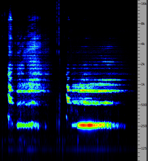
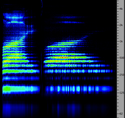
SOURCE
ORIGINAL
AUTO-CONVOLVED
SPECTRUM
Shakuhachi
(Randy Raine-Reusch)
note how the breathy aspects of
the sound have been muted
Bass singer
(Derek Christian)
note how the harmonics in the
voice become more prominent
(Click to enlarge)
Before we proceed, some cautionary comments.
Convolution is not a combination of EQ and
Reverb, which are both linear processes. EQ alters the
spectrum of a sound, but that is not done dynamically
as it would happen in a real space which has its own
complex frequency response where some frequencies are
damped and others brightened, and the overall duration
is extended. In other words, timbre and space are
intertwined in convolution just as they are in
the real world. Auto-convolution (AC)
then has a non-linear effect on the spectrum.
A simple example is that if the ratio of the strongest
frequency in the spectrum to a very weak frequency is
10:1, then by multiplying it with itself, that ratio
becomes 100:1 in the output spectrum. That is why it
was referred to earlier as a “thinning” of the
spectrum. Low level noisy components are gone. But the
price of this is that very large numbers are involved
in the calculations.
Therefore, the process of normalization is
absolutely needed in the process, which means that
whatever large values occur in the multiplication of
the spectrum, the overall output signal gets reduced
to the dynamic range of the output. In digital audio
(see the Sound-Medium
interface module on digital representation) a 24-bit
(or more) sample resolution is absolutely necessary to
avoid excess quantization at the lower
amplitude levels.
In fact, AC represents a “worst case scenario” for
convolution calculations. By definition the spectrum
is the same in the two signals being processed,
because they are the same sound. So therefore, the
strongest frequencies will get the maximum value in
the output. Even with normalization and the “floating
point” method of calculating large values, there still
may be a problem in dynamic range, so with very strong
sounds, it’s best to keep their maximum level at - 6dB
or less before using them in AC.
After hearing these stretched sounds,
it will be tempting to think that AC simply stretches
sounds. Of course it does, but things get more complex
when there are multiple sounds involved, such as
speech or a rhythmic sequence. Direct convolution, as
mentioned above, involves multiplying every sample
with every other sample in the file, and summing them
- clearly involving a lot of calculations. However, it
gives a clue as to what happens with multiple events.
Every individual sound is convolved with every
other sound in the sequence and summed.
For example, if there were ten sounds, the first would
be convolved with the first through to the 10th, then
the second sound would be treated the same, and
finally the last sound will be convolved with the
first through the last, and everything summed
together. The pattern then is the output starts and
ends simply, but gradually builds to the maximum
density in the middle, before thinning out again.
The density of the events in the output can be
controlled by using the Moving option which
refers to specifying a “Length Used” for the Impulse
signal. This length defaults to the entire length of
the Impulse, but a shorter specification, e.g. half,
means that the input sound will be processed with only
the first half of the Impulse, and then the second
half, thereby producing less density buildup. The
shorter the length used, the less the density. This
option isn’t very applicable for a sustained sound.
Vocal text auto-convolved (Christopher Gaze)
Finally, the AC process can be iterated multiple
times. For instance, the first iteration that doubles
the length can be the source for the same process, which
doubles the length again to four times, and continues to
thin out the spectrum to its principal components.
Sometimes a third iteration, stretching to 8 times,
still produces an interesting but very muted version. A
set of examples that have been used compositionally are
available here.
So, to summarize: AC emphasizes the strongest
frequencies in a spectrum and doubles the length of
the sound. Particularly when the sound is already
reverberant, the image suggested by the convolved sound
might seem half way between the original sound and the
reverberant sound. A bit more imaginatively, an
auto-convolved sound might seem more like a memory of
it, more muted and evocative, but you’ll have to
experience this for yourself.
D. Frequency Modulation
Synthesis.Frequency
Modulation (FM) is a standard non-linear
synthesis method. As noted above, with a single
sine-wave carrier and modulator, it is capable of
producing a wide range of spectra where the sidebands
are arranged in pairs around the carrier. As with Ring
Modulation, lower sidebands are reflected into
the positive domain when they go negative, and
specific frequency choices can result in both harmonic
and inharmonic spectra.
The chief advantage of the method, as originally
formulated by John Chowning at Stanford in the early
1970s, is that a single parameter, the Modulation
Index (I) controls the bandwidth of the
spectrum, instead of having to control the envelopes
of individual partials, as in Additive Synthesis. This
index is defined as the ratio between the amplitude
and frequency of the modulator, meaning that the
greater the amplitude of the modulator (its modulation
depth), the broader the bandwidth.
Putting an envelope onto the Modulation Index
produces a dynamic spectrum because the amplitude
changes in each sideband pair are non-synchronous, but
go through independent cycles of peaks and zeroes.
Although this lacks generality, it gives the aural
impression of a dynamically changing timbre similar to
actual musical notes. However, it can also simulate
percussive instruments and produce purely synthetic
timbres.
The key to understand simple FM (one carrier and one
modulator) is the theory behind the ratio of the
carrier to the modulator, the c:m ratio. It can
be studied in this Tutorial.
Multiple carrier and multiple modulator instruments
can also be designed. One specific use of the multiple
carrier, as developed by Chowning, is to simulate
vocal formants. By tuning the various carrier
frequencies to those associated with vocal formants,
and using a small modulation index, a formant-like
spectrum can be created.
FM synthesis became widely available with the Yamaha
DX7 keyboard synthesizer in the 1980s.
If
you would like to try some experiments with your
soundfiles similar to what is presented here, it’s
unlikely that any software you have will offer Ring
Modulation or Convolution. So, if not, download a
free copy of SoundHack from soundhack.com,
the site maintained by Tom Erbe of Cal Arts. He has
several free packages (under Freeware) of excellent
Mac plug-ins, plus some that you need to buy. But
the original SoundHack, which is almost 30 years old
now, is free and still available.
Note: SoundHack will only work with .aif
files (not .wav) on the Mac, except for Ring
Modulation.
Ring Modulation. The first
thing you’ll notice when you start SoundHack is that
nothing seems to happen! As you’ll see with the more
recent modules, Tom is perfectly capable of
providing a very intelligent and user friendly
interface, but the original SoundHack is pretty
basic. You need to start by opening a file (command
O) and then you’ll see it loaded and can proceed to
the Convolution option (command C) under the
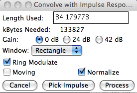
Hack menu. Try it first with the Ring
Modulation option which, as explained above, is
included in the Convolution option and looks like
this once you check the Ring Modulation box.
SoundHack
Ring Modulator
Of course, you’re going to need a second file called
the Impulse to modulate yours. If you have
any sine wave files, you can start with those as
long as their duration is the same or greater than
the file you want to modulate. If you’re handy with
Max/Msp, you can record some simple oscillators, but
if not, here is a set of files you can download
(right click or control click) of some useful
frequencies, and some sub-audio ones. They are
around 30” long.
I suggest starting with 100 Hz and 1 kHz as the
Impulse, similar to the above demo. There’s also 4
kHz and 8 kHz in case you’d like to try the
extreme transpositions they produce. And for
subaudio effects there’s a 6 Hz sine and square.
As noted in the diagram, use the Rectangular
window (which means using complete chunks of your
file) and always Normalize the output (for
maximum amplitude). Before you process the sound,
SoundHack will suggest a name for the output file,
but it’s probably better to simplify it to
something like BellX100Hz and then your choice of
filename extension and bit depth (16 bit will
suffice). SoundHack supports all the common
formats.
You can listen to it in the small bar at the
bottom by hitting the spacebar. If you like it,
then close the output file that’s on the
screen, look for it in your output folder and
import it into an editor for any cleanup that’s
needed. SoundHack tends to trim off any “zero
signal” that can occur when the impulse is longer
than the other signal, but not all programs will
do that.
If you want to try another version, make sure you
start by clicking again on your input file – which
is colourfully coded on the screen – with command
C in which case the word “Input” will
appear on it. Similarly you need to specify the Impulse
file again, and that word will also appear on it.
You can keep a lot of files open that you may want
to work with to modulate with each other. But,
again, in order to be able to edit the output
file in an editor, you have to close it in
SoundHack in order to avoid any confusion. But it
can be opened again if it’s needed for further
work.
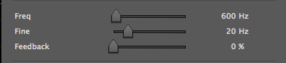
This is a simple (mda) Ring
Modulator plug-in that has a useful fine tuning
slider for frequency that ranges over 100 Hz only.
The main sine wave frequency is notched to 100 or
200 Hz steps, but sometimes is not very accurate,
such as the 100 Hz setting. A feedback level is
included that must be used carefully. However, it
gives a good range of effects and allows real-time
testing which is very valuable.
Personal
Studio Experiment No. 4
Auto-Convolution.
If you haven’t done so already, you probably should
download the Convolution
Techniques pdf, as it is very detailed about
all of the parameters used by SoundHack, and has
many tips and bits of advice on how to use it.
The basic approach proceeds similarly to Ring
Modulation (command C in the Hack menu), but the RM
box is not checked. Again, you start by loading a
file, or if it is already on the screen, click on it
to highlight it, then type Command C for Convolution
(or select it from the Hack menu). Make sure the
file now says “Input”. If not, start again. This box
will appear.
SoundHack
Convolution
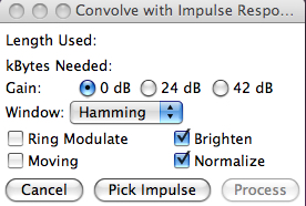
For auto-convolution (convolving a sound with
itself), you need a duplicate file for the
Impulse (the rule in SoundHack is that the two input
files must be different). The easiest way to do that
on a Mac is to highlight the file in the Finder and
type Command D. The duplicate file will have the
same name with “copy” added. The copy file can later
be deleted.
Select 0 dB to ensure the output the maximum dynamic
range, and Normalize as before. In this case, you
can select an analysis Window (e.g. Hamming). In the
pdf there’s more detail about what this means, but
for auto-convolution it shouldn’t make a difference.
We will return to this point when convolving two
separate files.
The Brighten option is often useful, and is
probably unique to SoundHack. In acoustic spectra,
it is typical that they fall off at 6-9 dB per
octave. However, auto-convolution emphasizes the
strongest frequencies, so it is entirely possible
that the highs will be quite dull in the output if
you don’t use Brighten which boosts the high
frequencies by 6 dB/octave.
On the other hand, if the sound is very strong in
the highs already, you don’t need to use it.
Sometimes you need to do the Convolution twice, once
with and once without Brighten just to see the
effect (put something like NB on the filename if
it’s not brightened). Keep in mind, you can always
EQ the file later.
Then you select the Impulse file (the copy
of the original) and process. Again SoundHack will
suggest a name based on the two files, but it’s
better to keep it simple like Bell*self plus
the extension. On the other hand, it’s possible
another program will object to the use of the *
character in the filename. Of course, that’s
ridiculous because it’s the correct mathematical
symbol, but software designers don’t like “special
characters” even when they’re accurate descriptors.
The most important thing to remember is that you
must use a 24 bit format for the output – this
is unfortunately not the default. So if you
accidentally let the 16-bit format be calculated,
you’ll have to re-do the process as you’ll get a lot
of quantizing noise.
It’s best to use shorter sounds during your
experimental phase (10-20 sec), but with today’s
processors, the calculation are still quite speedy.
You can always edit a short bit out of a longer file
to do some testing. Convolution is always
trial-and-error, so be patient. If the calculation
is long, you’ll see a whirling bullseye indicating
the processing is still going on.
Once the calculation is done, the output file will
appear on the screen in a new colour and you can
play it by hitting the spacebar, just to see if it
seems to have turned out alright. Even if the answer
is yes, close it on the screen, and open it in an
editor. There will almost always be things to check.
First of all, there may be extraneous silences at
the beginning and usually at the end; these may be
excised, particularly if you’re going to repeat the
AC for another iteration and doubling. Also check
the levels of the left and right channels. Since all
amplitudes get exaggerated, any small difference in
the original L/R balance will be exaggerated in the
output. Select either the stronger channel to reduce
its level, or the weaker one to increase it, and
make sure you know how to do this on your editor. If
you’re planning on iterating the AC, this imbalance
will just get worse otherwise. Then save the revised
file.
There is one known bug in SoundHack which
occasionally appears. In the normalization process,
a single sample can actually go over the
maximum range and come out as maximum negative,
producing a nasty click. There are two remedies:
expand the file in your editor and micro-edit out
the incorrect sample (yes, some editors make that
easy to do, others not). Otherwise, go back and try
a different analysis window, e.g. Rectangular.
Chances are the error won’t occur this time. If
there is a “legitimate” amplitude overflow, not just
one sample, go back and reduce the amplitude of your
input file by 6 dB.
If you’d like to auto-convolve the file again, make
another copy (Command D), and go back to SoundHack
and open the convolved file and repeat the process.
This time the Impulse will be the copy of the first
convolved file. Note that not all the menu settings
will remain the same as before, so check them over,
particularly the bit rate.
If for some reason, you’re not happy with the
process of stretching by 2, 4, 8, etc., there are
other options. If we can refer to the original file
as 1 and the auto-convolved file as 2, then
convolving them is 2+1=3 times longer. Similarly 4+2
equals 6 times longer and so on. It’s tricky to keep
this all straight, so good file naming is essential.
In the previous module, we looked at the classic
analog parallel circuit where multiple
synchronized versions of a sound could be
processed separately and then mixed together. We
tried to replicate this with a ProTools session
where we recorded (i.e. latched) the playback
levels to create a dynamic mix. Then we did
something similar in non-real-time, by
assembling a small mixing session where the
individual tracks were already processed and
then mixed with amplitude breakpoints. Both of
these solutions can of course be extended with
files that are non-synchronous, but perhaps
still related.
During those demo’s we spoke about performability,
involving real-time processing that could be
recorded – something that was taken for granted
in the analog studio. We also noted that some
plug-ins, such as GRM Tools were specifically
well designed to replicate that kind of freedom
because of the efficient real-time controls,
using presets and ramps that interpolated
between them, along with the x-y mouse control
for controlling two parameters at once.
But we also noted the common pitfall in plug-ins
in terms of whether dynamic processing created audible
artifacts such as clicks while parameters
were being adjusted. Two processes that are very
difficult to design without those artifacts are
certain filter settings, as in the previous
module, and time delays, as covered in the next
one.
The advantage of being able to “perform” this
kind of processing in real-time is that, just as
in the analog studio, you can control the
processing in response to the sound itself and
hence create a correlation appropriate
to its own character and gestures. This can also
be referred to as “hand-ear” correlation, which
when done intelligently often makes it seem like
the sound is changing of its own accord, as
opposed to being arbitrarily manipulated.
The choice is a matter of taste and intent, and
could work either way, but in general, the
former approach (integrating the processing with
the sound), gives a more organic feel to the
result, and doesn’t draw the listener’s
attention to the manipulation. The latter
approach, being more arbitrary and uncorrelated,
does the opposite, which might still mean
something to the listener. Very few digital
processes allow the processing to be influenced
by the behaviour of the signal itself. The
easiest correlation to make is with an amplitude
follower (or envelope follower) where the
signal’s amplitude can determine the strength of
a process, for instance.
The disadvantage of this form of digital
performability is that it doesn’t usually fit
the model of the DAW which is mainly designed
for assembling and controlling a mix in
non-real-time, then bouncing it to a finished
soundfile. There are some solutions to this
problem, but most are not very practical or
available.
- a standalone app might
include a direct-to-disk option
(such as MacPod that will be introduced
later); once the user starts a recording and
begins to manipulate the sound, everything
that happens to the sound will be recorded.
This facilitates improvisation, taking risks
– and later discarding anything not worth
saving.
- following analog practice,
the “live” performance with a plug-in can
simply be recorded – but where and
how? Well if you have two computers, there's
no problem in connecting them; likewise if
you have two audio interfaces, a digital
patch out of one to the input of the other
can be arranged. Either of those situations
today is a luxury.
- if we’re willing to give up
the freedom of total improvisation to
something more “rehearsed”, then we can use
the same resources that we saw previously in
the ProTools parallel circuit using
Auxiliaries and Inserts. Once the
parameter(s) involved in the process are
specified for “automation” on a
specific track, we can see its values on a
separate line in Edit Mode, similar to
Volume. Then we can “latch” that
parameter, perform the dynamic change of the
parameter during playback, with the result
being stored. Afterwards, any subsection can
be re-done with the “touch” mode
where stored values are over-written by any
manually triggered gestures.
Here’s a specific example,
extending the parallel Auxiliary patch from
the previous module. To keep things simple, we
are going to change the cut-off frequency in
the left and right high-pass and low-pass
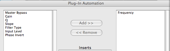
filters assigned to them. First we activate
the Automation button on the plug-in
(shown below as Auto mode), and select the
parameter to be controlled using the Add
button, like this.
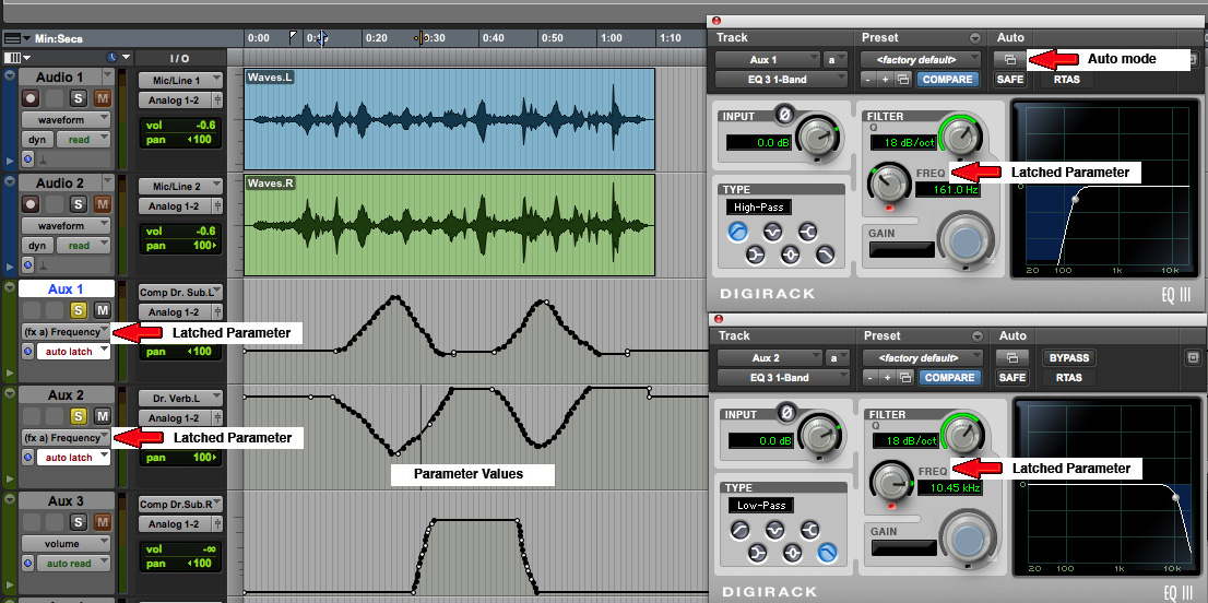
Then we set up the latching
mechanism as shown and do the recording. At
this point, we illustrate two choices for how
to do this with a mouse, similar to how mixing
levels are recorded – one track (or multiple
ones grouped together) at a time, or by
real-time switching between the levels of
different tracks. Of course, if you’re lucky
enough to have a (physical) digital mixer
attached to the DAW, you don’t need to
compromise on this point.
(click to enlarge)
Dynamically
filtered waves
(click to enlarge)
Dynamically
filtered waves
In the left hand example, we alternately
controlled the left channel process and then the
right channel process via the mouse. This
created a pseudo-stereo panning
effect which was accomplished with one pass. In
the right hand example, we recorded the left
channel control first, then re-cued the track to
record the right channel control (while
listening to the left channel by including it in
the Solo monitor).
The aural result is that the quasi
synchronization of our performance of both
cutoff frequencies gave the impression of the
changes happening to the entire sound, not its
L/R components. Note that, given the nature of
the controls going in opposite directions, this
pattern could not be achieved at the same time.
Is one version preferable to the other – you
decide for yourself!
Q. Try this review quiz to
test your comprehension of the above material,
and perhaps to clarify some distinctions you may
have missed. Note that a few of the questions
may have "best" and "second best" answers to
explain these distinctions.