Postscript version of this file

STAT 380 Lecture 3

Reading for Today's Lecture: Chapters 1, 2 and 3 of Ross.

Today's lecture Summary

• Example to review
  • basic probability: sample space, events, random variables, expected value

  • standard distributions: Binomial, Geometric, Poisson

  • conditional probability, independence

  • Baye's rule

• Introduce first step analysis

Example 3: Survival of family names. Traditionally: family name follows sons. Given man at end of 20th century. Probability descendant (male) with same last name alive at end of 21st century? or end of 30th century?

Simplified model: count generations not years. Compute probability, of survival of name for n generations.

Technically easier to compute q_n, probability of extinction by generation n.

Useful rvs:

$$X= \text{\char93 of male children of first man}$$

$$Z_k = \text{\char93 of male children in generation $k$}$$

Event of interest:

$$E_n = \{ Z_n=0\}$$

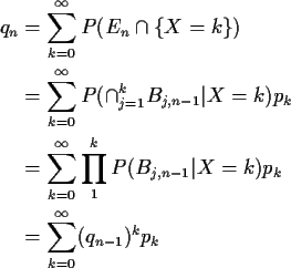
Break up E_n:

$$q_n=P(E_n) = \sum_{k=0}^\infty P(E_n\cap \{ X=k\})$$

Now look at the event $E_n\cap \{ X=k\}$. Let
$$\begin{align*}B_{j,n-1} =& \{ X=k\}\cap \{\text{child $j$ s line extinct} \\ & \quad \text{ in $n-1$\space generations}\} \end{align*}$$
Then

$$E_n\cap \{ X=k\} =\cap_{j=1}^k B_{j,n-1}$$

Now add modelling assumptions:

1.

Given (conditional on) X=k the events B_j,n-1 are independent. In other words: one son's descendants don't affect other sons' descendants.

2.

Given X=k the probability of B_j,n-1 is q_n-1. In other words: sons are just like the parent.

Now add notation P(X=k) = p_k.
$$\begin{align*}q_n & = \sum_{k=0}^\infty P(E_n\cap \{ X=k\}) \\ & = \sum_{k=0}^\... ...P(B_{j,n-1}\vert X=k) p_k \\ & = \sum_{k=0}^\infty (q_{n-1})^k p_k \end{align*}$$
Probability generating function:

$$\phi(s) = \sum_{k=0}^\infty s^k p_k = {\rm E}(s^X)$$

We have found

q₁ = p₀

and

$$q_n = \phi(q_{n-1})$$

Notice that $q_1 \le q_2 \le \cdots$ so that the limit of the q_n, say $q_\infty$, must exist and (because $\phi$ is continuous) solve

$$q_\infty = \phi(q_\infty)$$

Special cases

Geometric Distribution: Assume

$$P(X=k) = (1-\theta)^k \theta \qquad k=0,1,2,\ldots$$

(X is number of failures before first success. Trials are Bernoulli; $\theta$ is probability of success.)

Then
$$\begin{align*}\phi(s) & = \sum_0^\infty s^k (1-\theta)^k \theta \\ & = \theta \... ...fty \left[s(1-\theta)\right]^k \\ & = \frac{\theta}{1-s(1-\theta)} \end{align*}$$
Set $\phi(s) = s$ to get

$$s[1-s(1-\theta)]=\theta$$

Two roots are

$$\frac{1 \pm \sqrt{1-4\theta(1-\theta)}}{2(1-\theta)} = \frac{1 \pm (1-2\theta)}{2(1-\theta)}$$

One of the roots is 1; the other is

$$\frac{\theta}{1-\theta}$$

If $\theta \ge 1/2$ the only root which is a probability is 1 and $q_\infty=1$. If $\theta < 1/2$ then in fact $q_n \to q_\infty = \theta/(1-\theta)$.

Binomial($m,\theta$): If

$$P(X=k) = \binom{m}{k} \theta^k(1-\theta)^{m-k} \quad k=0,\ldots, m$$

then
$$\begin{align*}\phi(s) & = \sum_0^m \binom{m}{k} (s\theta)^k(1-\theta)^{m-k} \\ & = (1-\theta+s\theta)^m \end{align*}$$
The equation $\phi(s) = s$ has two roots. One is 1. The other is less than 1 if and only if $m\theta={\rm E}(X) > 1$.

Poisson($\lambda$): Now

$$P(X=k) = e^{-\lambda} \lambda^k/k! \quad k=0,1,\ldots$$

and

$$\phi(s) = e^{\lambda(s-1)}$$

The equation $\phi(s) = s$ has two roots. One is 1. The other is less than 1 if and only if $\lambda = {\rm E}(X) > 1$.

Important Points:

• Use of conditioning.

• Approximate nature of modelling assumptions

• Key assumptions of conditional independence, homogeneity