![]()
![]()
![]()
Reading for Today's Lecture: Chapter 3
Goals of Today's Lecture:
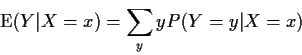
Conditional Expectations
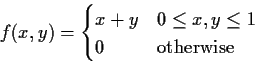
If X, Y, two discrete random variables then
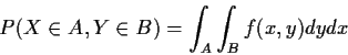
Extension to absolutely continuous case:
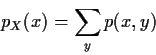
Joint pmf of X and Y is defined as
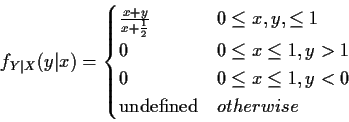
Example:
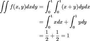
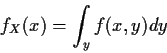
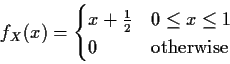
The marginal density of X is, for
![]() .
.
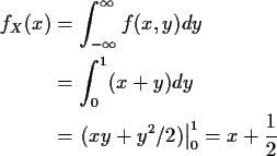
For x not in [0,1] the integral is 0 so
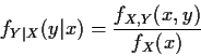
Conditional Densities
If X and Y have joint density
fX,Y(x,y) then
we define the conditional density of Y given X=x by
analogy with our interpretation of densities. We take limits:
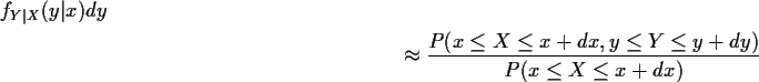
in the sense that if we divide through by dy and let
dx and dy tend to 0 the conditional density is the limit

Going back to our interpretation of joint densities and ordinary
densities we see that our definition is just
Example: For f of previous example conditional density
of Y given X=x defined only for
![]() :
:

WARNING: in sum
![]() is required and x, y integers
so sum really runs from y to
is required and x, y integers
so sum really runs from y to ![]()
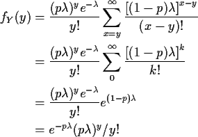
which is a Poisson(![]() )
distribution.
)
distribution.
Conditional Expectations
If X and Y are continuous random variables with joint density
fX,Y we define:
Key properties of conditional expectation
1: If ![]() then
then
![]() .
Equals iff
P(Y=0|X=x)=1.
.
Equals iff
P(Y=0|X=x)=1.
2:
![]() .
.
3: If Y and X are independent then
4:
![]() .
.