Postscript version of this file

STAT 380 Lecture 8

Reading for Today's Lecture: Chapter 4 sections 1-3.

Goals of Today's Lecture:

• Define Markov Chain.

• Introduce transition matrix

• Derive Chapman Kolmogorov equations.

Look at the matrix product ${\bf P}{\bf P}$:

$$\left[\begin{array}{ll} \frac{3}{5} & \frac{2}{5} \\ \frac{1... ... \frac{2}{5} \\ \frac{1}{5} & \frac{4}{5} \end{array} \right]$$

Notice that the probability P(X₂=W|X₀=W) is exactly the formula for the W,W entry in ${\bf P}{\bf P}$.

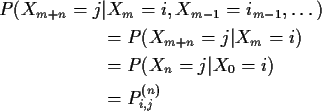
General case. Define

P⁽ⁿ⁾_i,j =P(X_n=j|X₀=i)

Then
$$\begin{align*}P(X_{m+n}=j &\vert X_m=i, X_{m-1}=i_{m-1},\ldots) \\ & = P(X_{m+n}=j\vert X_m=i) \\ & =P(X_n=j\vert X_0=i) \\ & = P^{(n)}_{i,j} \end{align*}$$

Proof of these assertions by induction on m,n.

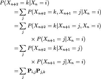
Example for n=2. Two bits to do:

First suppose U,V,X,Y are discrete variables. Assume
$$\begin{align*}P(Y=y\vert X=x,&U=u,V=v) \\ & = P(Y=y\vert X=x) \end{align*}$$
for any x,y,u,v. Then I claim
$$\begin{align*}P(Y=y &\vert X=x,U=u) \\ &= P(Y=y\vert X=x) \end{align*}$$
In words, if knowing both U and V doesn't change the conditional probability then knowing U alone doesn't change the conditional probability.

Proof of claim:

$$A=\{X=x,U=u\}$$

Then
$$\begin{align*}P(Y=y &\vert X=x,U=u) \\ & = \frac{P(Y=y,A)}{P(A)} \\ & = \frac{... ...} \\ & = \frac{ P(Y=y\vert X=x)P(A)}{P(A)} \\ &= P(Y=y\vert X=x) \end{align*}$$

Second step: consider
$$\begin{align*}P(X_{n+2}& =k \vert X_n=i) \\ = & \sum_j P(X_{n+2}=k,X_{n+1}=j\v... ...mes P(X_{n+1}=j\vert X_n=i) \\ =& \sum_j {\bf P}_{i,j}{\bf P}_{j,k} \end{align*}$$
This shows that

$$P(X_{n+2}=k\vert X_n=i) = ({\bf P}^2)_{i,k}$$

where ${\bf P}^2$ means the matrix product ${\bf P}{\bf P}$. Notice both that the quantity does not depend on n and that we can compute it by taking a power of ${\bf P}$.

More general version

$$P(X_{n+m}=k\vert X_n=j) = ({\bf P}^m)_{j,k}$$

Since ${\bf P}^n{\bf P}^m={\bf P}^{n+m}$ we get the Chapman-Kolmogorov equations:
$$\begin{multline*}P(X_{n+m}=k\vert X_0=i) = \\ \sum_j P(X_{n+m}=k\vert X_n=j)P(X_n=j\vert X_0=i) \end{multline*}$$

Summary: A Markov Chain has stationary n step transition probabilities which are the nth power of the 1 step transition probabilities.

Here is Maple output for the 1,2,4,8 and 16 step transition matrices for our rainfall example:

> p:= matrix(2,2,[[3/5,2/5],[1/5,4/5]]);
                      [3/5    2/5]
                 p := [          ]
                      [1/5    4/5]
> p2:=evalm(p*p):
> p4:=evalm(p2*p2):
> p8:=evalm(p4*p4):
> p16:=evalm(p8*p8):

This computes the powers (evalm understands matrix algebra).

Fact:

$$\lim_{n\to\infty} {\bf P}^n = \left[ \begin{array}{cc} \frac{... ...{3} \\ \\ \frac{1}{3} & \frac{2}{3} \end{array}\right] \, .$$

> evalf(evalm(p));
            [.6000000000    .4000000000]
            [                          ]
            [.2000000000    .8000000000]
> evalf(evalm(p2));
            [.4400000000    .5600000000]
            [                          ]
            [.2800000000    .7200000000]
> evalf(evalm(p4));
            [.3504000000    .6496000000]
            [                          ]
            [.3248000000    .6752000000]
> evalf(evalm(p8));
            [.3337702400    .6662297600]
            [                          ]
            [.3331148800    .6668851200]
> evalf(evalm(p16));
            [.3333336197    .6666663803]
            [                          ]
            [.3333331902    .6666668098]

Where did 1/3 and 2/3 come from?

Suppose we toss a coin $P(H)=\alpha_D$ and start the chain with Dry if we get heads and Wet if we get tails.

Then

$$P(X_0=x) = \begin{cases}\alpha_D & x=\text{Dry} \\ \alpha_W=1-\alpha_D & x=\text{Wet} \end{cases}$$

and
$$\begin{align*}P(X_1=x) & = \sum_y P(X_1=x\vert X_0=y)P(X_0=y) \\ & = \sum_y \alpha_y P_{y,x} \, . \end{align*}$$
Notice last line is a matrix multiplication of row vector $\alpha$ by matrix ${\bf P}$.

A special $\alpha$: if we put $\alpha_D=1/3$ and $\alpha_W=2/3$ then

$$\left[ \frac{1}{3} \quad \frac{2}{3} \right] \left[\begin{ar... ...y} \right] = \left[ \frac{1}{3} \quad \frac{2}{3} \right] \, .$$

In other words if we start off P(X₀=D)=1/3 then P(X₁=D)=1/3and analogously for W. This means that X₀ and X₁ have the same distribution.

A probability vector $\alpha$ is called an initial distribution for the chain if

$$P(X_0=i) = \alpha_i \, .$$

A Markov Chain is stationary if

P(X₁=i) = P(X₀=i)

for all i.

An initial distribution is called stationary if the chain is stationary. We find that $\alpha$ is a stationary initial distribution if

$$\alpha {\bf P}=\alpha \, .$$

Suppose ${\bf P}^n$ converges to some matrix ${\bf P}^\infty$. Notice that

$$\lim_{n\to\infty} {\bf P}^{n-1} = {\bf P}^\infty$$

and
$$\begin{align*}{\bf P}^\infty & = \lim {\bf P}^n \\ & = \left[\lim {\bf P}^{n-1}\right] {\bf P} \\ & = {\bf P}^\infty {\bf P}\, . \end{align*}$$

This proves that each row $\alpha$ of ${\bf P}^\infty$ satisfies

$$\alpha = \alpha {\bf P}\, .$$

Def'n: A row vector x is a left eigenvector of A with eigenvalue $\lambda$ if

$$xA=\lambda x \, .$$

So each row of ${\bf P}^\infty$ is a left eigenvector of ${\bf P}$ with eigenvalue 1.