Postscript version of this page

STAT 801: Mathematical Statistics

Monte Carlo

Given random variables $X_1,\ldots,X_n$ whose joint density $f$ (or distribution) is specified and a statistic $T(X_1,\ldots,X_n)$ whose distribution you want to know. To compute something like $P(T > t)$:

1. Generate $X_1,\ldots,X_n$ from the density $f$.

   
   

2. Compute $T_1 = T(X_1,\ldots,X_n)$.

   
   

3. Repeat $N$ times getting $T_1, \ldots,T_N$.

   
   

4. Estimate $p=P(T>t)$ as $\hat p =M/N$ where $M$ is number of repetitions where $T_i >t$.

   
   

5. Estimate accuracy of $\hat p$ using $\sqrt{\hat p ( 1 - \hat p)/N}$.

Notice accuracy inversely proportional to $\sqrt{N}$. There are a number of tricks to make the method more accurate (but they only change the constant of proportionality - the SE is still inversely proportional to the square root of the sample size).

Generating the Sample

Transformation

Most computer languages have a facility for generating pseudo uniform random numbers, that is, variables $U$ which have (approximately of course) a Uniform$[0,1]$ distribution. Other distributions are generated by transformation:

Exponential: $X=-\log U$ has an exponential distribution:

$$P(X > x) = P(-\log(U) > x)$$

$$= P(U \le e^{-x})=e^{-x}$$

Random uniforms generated on the computer sometimes have only 6 or 7 digits or so of detail. This can make the tail of your distribution grainy. If $U$ were actually a multiple of $10^{-6}$ for instance then the largest possible value of $X$ is $6\log(10)$. This problem can be ameliorated by the following algorithm:

• Generate $U$ a Uniform[0,1] variable.

• Pick a small $\epsilon$ like $10^{-3}$ say. If $U>\epsilon$ take $Y=-\log(U)$.

• If $U \le \epsilon$ remember that the conditional distribution of $Y-y$ given $Y>y$ is exponential. You use this by generating a new $U^\prime$ and computing $Y^\prime=-\log(U^\prime)$. Then take $Y=Y^\prime -\log(\epsilon)$. The resulting $Y$ has an exponential distribution. You should check this by computing $P(Y > y)$.

General technique: inverse probability integral transform.

If $X$ is to have cdf $F$:

Generate $U\sim Uniform[0,1]$.

Take $X=F^{-1}(U)$:

$$P(Y \le y) = P(F^{-1}(U) \le y)$$

$$= P(U \le F(y))= F(y)$$

Example: $X$ exponential. $F(x)= 1-e^{-x}$ and $F^{-1}(u) = -\log(1-u)$.

Compare to previous method. (Use $U$ instead of $1-U$.)

Normal: $F=\Phi$ (common notation for standard normal cdf).

No closed form for $F^{-1}$.

One way: use numerical algorithm to compute $F^{-1}$.

Alternative: Box Müller

Generate $U_1,U_2$ two independent Uniform[0,1] variables.

Define

$$Y_1 = \sqrt{-2\log(U_1)} \cos(2\pi U_2)$$

and

$$Y_2 = \sqrt{-2\log(U_1)} \sin(2\pi U_2)\, .$$

Exercise: (use change of variables) $Y_1$ and $Y_2$ are independent $N(0,1)$ variables.

Acceptance Rejection

Suppose: can't calculate $F^{-1}$ but know $f$.

Find density $g$ and constant $c$ such that

1. $f(x) \le cg(x)$ for each $x$ and

2. $G^{-1}$ is computable or can generate observations $W_1, W_2, \ldots$ independently from $g$.

Algorithm:

1. Generate $W_1$.

2. Compute $p=f(W_1)/(cg(W_1)) \le 1$.

3. Generate uniform[0,1] random variable $U_1$ independent of all $W$s.

4. Let $Y=W_1$ if $U_1 \le p$.

5. Otherwise get new $W, U$; repeat until you find $U_i \le f(W_i)/(cg(W_i))$.

6. Make $Y$ be last $W$ generated.

This $Y$ has density $f$.

Markov Chain Monte Carlo

Recently popular tactic, particularly for generating multivariate observations.

Theorem Suppose $W_1, W_2, \ldots$ is an (ergodic) Markov chain with stationary transitions and the stationary initial distribution of $W$ has density $f$. Then starting the chain with any initial distribution

$$\frac{1}{n} \sum_{i=1}^n g(W_i) \to \int g(x) f(x) dx \, .$$

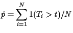
Estimate things like $\int_A f(x) dx$ by computing the fraction of the $W_i$ which land in $A$.

Many versions of this technique including Gibbs Sampling and Metropolis-Hastings algorithm.

Technique invented in 1950s: Metropolis et al.

One of the authors was Edward Teller ``father of the hydrogen bomb''.

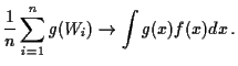
Importance Sampling

If you want to compute

$$\theta \equiv E(T(X)) = \int T(x) f(x) dx$$

you can generate observations from a different density $g$ and then compute

$$\hat\theta = n^{-1} \sum T(X_i) f(X_i)/g(X_i)$$

Then

$$E(\hat\theta) = n^{-1} \sum E\left\{T(X_i) f(X_i)/g(X_i)\right\}$$

$$= \int \{T(x) f(x)/g(x)\} g(x) dx$$

$$= \int T(x) f(x) dx$$

$$= \theta$$

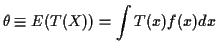
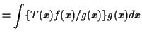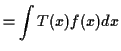Variance reduction

Consider the problem of estimating the distribution of the sample mean for a Cauchy random variable. The Cauchy density is

$$f(x) = \frac{1}{\pi(1+x^2)}$$

We generate $U_1, \ldots, U_n$ uniforms and then define $X_i = \tan^{-1}(\pi(U_i-1/2))$. Then we compute $T=\bar{X}$. Now to estimate $p=P(T>t)$ we would use

$$\hat p = \sum_{i=1}^N 1(T_i > t) /N$$

after generating $N$ samples of size $n$. This estimate is unbiased and has standard error $\sqrt{p(1-p)/N}$.

We can improve this estimate by remembering that $-X_i$ also has Cauchy distribution. Take $S_i=-T_i$. Remember that $S_i$ has the same distribution as $T_i$. Then we try (for $t>0$)

$$\tilde p = [\sum_{i=1}^N 1(T_i > t) + \sum_{i=1}^N 1(S_i > t) ]/(2N)$$

which is the average of two estimates like $\hat p$. The variance of $\tilde p$ is

$$\begin{multline*} (4N)^{-1} Var(1(T_i > t)+1(S_i > t)) \\ = (4N)^{-1} Var( 1(\vert T\vert > t)) \end{multline*}$$

which is

$$\frac{2p(1-2p)}{4N} = \frac{p(1-2p)}{2N}$$

Notice that the variance has an extra 2 in the denominator and that the numerator is also smaller - particularly for $p$ near 1/2. So this method of variance reduction has resulted in a need for only half the sample size to get the same accuracy.

Regression estimates

Suppose we want to compute

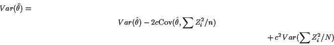
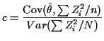
$$\theta = E(\vert Z\vert)$$

where $Z$ is standard normal. We generate $N$ iid $N(0,1)$ variables $Z_1,\ldots,Z_N$ and compute $\hat\theta = \sum\vert Z_i\vert/N$. But we know that $E(Z_i^2) = 1$ and can see easily that $\hat\theta$ is positively correlated with $\sum Z_i^2 / N$. So we consider using

$$\tilde\theta = \hat\theta -c(\sum Z_i^2/N-1)$$

Notice that $E(\tilde\theta) = \theta$ and

$$\begin{multline*} Var(\tilde\theta) = \\ Var(\hat\theta) -2c {\rm Cov}(\hat\theta, \sum Z_i^2/n) \\ +c^2 Var(\sum Z_i^2/N) \end{multline*}$$

The value of $c$ which minimizes this is

$$c=\frac{{\rm Cov}(\hat\theta, \sum Z_i^2/n)}{Var(\sum Z_i^2/N)}$$

and this value can be estimated by regressing the $\vert Z_i\vert$ on the $Z_i^2$!