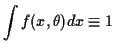
![]()
![]()
![]()
The problem above illustrates a general phenomenon. An estimator can
be good for some values of ![]() and bad for others. When comparing
and bad for others. When comparing
![]() and
and
![]() , two estimators of
, two estimators of ![]() we will say
that
we will say
that
![]() is better than
is better than
![]() if it has uniformly
smaller MSE:
if it has uniformly
smaller MSE:
The definition raises the question of the existence of a best
estimate - one which is better than every other estimator. There is
no such estimate. Suppose
![]() were such a best estimate. Fix
a
were such a best estimate. Fix
a ![]() in
in ![]() and let
and let
![]() . Then the
MSE of
. Then the
MSE of ![]() is 0 when
is 0 when
![]() . Since
. Since
![]() is
better than
is
better than ![]() we must have
we must have
Principle of Unbiasedness: A good estimate is unbiased, that is,
WARNING: In my view the Principle of Unbiasedness is a load of hog wash.
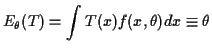
For an unbiased estimate the MSE is just the variance.
Definition:
An estimator ![]() of a parameter
of a parameter
![]() is
Uniformly Minimum Variance Unbiased (UMVU) if, whenever
is
Uniformly Minimum Variance Unbiased (UMVU) if, whenever
![]() is an unbiased estimate of
is an unbiased estimate of ![]() we have
we have
The point of having
![]() is to study problems like estimating
is to study problems like estimating
![]() when you have two parameters like
when you have two parameters like ![]() and
and ![]() for example.
for example.
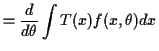
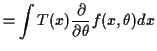
If
![]() we can derive some information from the
identity
we can derive some information from the
identity
 |
||
 |
||
 |
||
Summary of Implications
What can we do to find UMVUEs when the CRLB is a strict inequality?
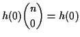
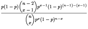
Example: Suppose ![]() has a Binomial(
has a Binomial(![]() ) distribution.
The score function is
) distribution.
The score function is
Different tactic: Suppose
![]() is some unbiased function of
is some unbiased function of ![]() . Then we have
. Then we have
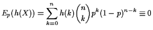
A Binomial random variable is a sum of ![]() iid Bernoulli
iid Bernoulli![]() rvs. If
rvs. If
![]() iid Bernoulli(
iid Bernoulli(![]() ) then
) then
![]() is Binomial(
is Binomial(![]() ). Could we do better by than
). Could we do better by than
![]() by trying
by trying
![]() for some other function
for some other function ![]() ?
?
Try ![]() . There are 4 possible values for
. There are 4 possible values for
![]() . If
. If
![]() then
then
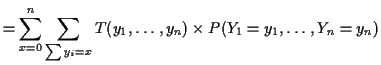
![$\displaystyle E_p( [T(Y_1,\ldots,Y_n)-X/n][X/n-p])
=\sum_{y_1,\ldots,y_n}
[T(y_1,\ldots,y_n)-\sum y_i/n][\sum y_i/n -p]
\times p^{\sum y_i} (1-p)^{n-\sum
y_i}
$](img115.gif)
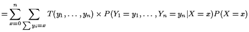
![$\displaystyle = \sum_{x=0}^n \sum_{\sum y_i=x} [T(y_1,\ldots,y_n)-\sum y_i/n] [\sum y_i/n -p] p^{\sum y_i} (1-p)^{n-\sum y_i}$](img119.gif) |
||
![$\displaystyle = \sum_{x=0}^n \left[ \sum_{\sum y_i=x} [T(y_1,\ldots,y_n)-x/n]\right][x/n -p] \times p^{x} (1-p)^{n-x}$](img120.gif) |
We have already shown that the sum in ![]() is 0!
is 0!
This long, algebraically involved, method of proving that
![]() is the UMVUE of
is the UMVUE of ![]() is one special case of
a general tactic.
is one special case of
a general tactic.
To get more insight rewrite
 |
||
 |
||
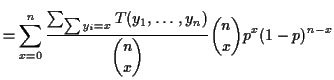 |
Notice large fraction in formula is average value
of ![]() over values of
over values of ![]() when
when ![]() is held fixed at
is held fixed at ![]() . Notice
that the weights in this average do not depend on
. Notice
that the weights in this average do not depend on ![]() . Notice that
this average is actually
. Notice that
this average is actually

Notice: with data
![]() log likelihood
is
log likelihood
is
In the binomial situation the conditional distribution of the data
![]() given
given ![]() is the same for all values of
is the same for all values of ![]() ; we
say this conditional distribution is free of
; we
say this conditional distribution is free of ![]() .
.
Defn: Statistic ![]() is sufficient for the model
is sufficient for the model
![]() if conditional distribution of
data
if conditional distribution of
data ![]() given
given ![]() is free of
is free of ![]() .
.
Intuition: Data tell us about ![]() if
different values of
if
different values of ![]() give different distributions to
give different distributions to ![]() . If two
different values of
. If two
different values of ![]() correspond to same density or cdf
for
correspond to same density or cdf
for ![]() we cannot distinguish these two values of
we cannot distinguish these two values of
![]() by examining
by examining ![]() . Extension of this notion: if two
values of
. Extension of this notion: if two
values of ![]() give same conditional distribution of
give same conditional distribution of ![]() given
given ![]() then observing
then observing ![]() in addition to
in addition to ![]() doesn't improve our ability to
distinguish the two values.
doesn't improve our ability to
distinguish the two values.
Mathematically Precise version of this intuition: Suppose ![]() is sufficient statistic and
is sufficient statistic and ![]() is any
estimate or confidence interval or ... If you only
know value of
is any
estimate or confidence interval or ... If you only
know value of ![]() then:
then:
You can carry out the first step only if the statistic ![]() is
sufficient; otherwise you need to know the true value of
is
sufficient; otherwise you need to know the true value of ![]() to
generate
to
generate ![]() .
.
Example 1:
![]() iid Bernoulli(
iid Bernoulli(![]() ).
Given
).
Given
![]() the indexes of the
the indexes of the ![]() successes have the
same chance of being any one of the
successes have the
same chance of being any one of the
![]() possible subsets of
possible subsets of
![]() . Chance does not depend on
. Chance does not depend on ![]() so
so
![]() is sufficient statistic.
is sufficient statistic.
Example 2:
![]() iid
iid ![]() .
Joint distribution of
.
Joint distribution of
![]() is MVN.
All entries of mean vector are
is MVN.
All entries of mean vector are ![]() . Variance covariance
matrix partitioned as
. Variance covariance
matrix partitioned as
![$\displaystyle \left[\begin{array}{cc} I_{n \times n} & {\bf 1}_n /n
\\
{\bf 1}_n^t /n & 1/n \end{array}\right]
$](img142.gif)
Compute conditional means and variances of ![]() given
given
![]() ; use fact that conditional law is MVN.
Conclude conditional law of data given
; use fact that conditional law is MVN.
Conclude conditional law of data given
![]() is MVN. Mean vector has all
entries
is MVN. Mean vector has all
entries ![]() . Variance-covariance matrix is
. Variance-covariance matrix is
![]() . No dependence
on
. No dependence
on ![]() so
so
![]() is sufficient.
is sufficient.
WARNING: Whether or not statistic is sufficient depends on
density function and on ![]() .
.
Theorem: [Rao-Blackwell] Suppose ![]() is a sufficient statistic
for model
is a sufficient statistic
for model
![]() . If
. If ![]() is an
estimate of
is an
estimate of
![]() then:
then:
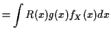
Proof: Review conditional distributions: abstract definition of conditional expectation is:
Defn: ![]() is any function of
is any function of ![]() such that
such that
Fact: If ![]() has joint density
has joint density
![]() and
conditional density
and
conditional density ![]() then
then

Proof:
 |
||
 |
||
 |
||
Think of ![]() as
average
as
average ![]() holding
holding ![]() fixed. Behaves like ordinary
expected value but functions of
fixed. Behaves like ordinary
expected value but functions of ![]() only are like constants:
only are like constants:
Example:
![]() iid Bernoulli(
iid Bernoulli(![]() ). Then
). Then
![]() is Binomial(
is Binomial(![]() ). Summary of conclusions:
). Summary of conclusions:
This proof that
![]() is UMVUE of
is UMVUE of ![]() is special case of
general tactic.
is special case of
general tactic.
Proof of the Rao Blackwell Theorem
Step 1: The definition of sufficiency is that the
conditional distribution of ![]() given
given ![]() does not depend on
does not depend on
![]() . This means that
. This means that ![]() does not depend on
does not depend on ![]() .
.
Step 2: This step hinges on the following identity (called Adam's law by Jerzy Neyman - he used to say it comes before all the others)
From this we deduce that
Step 3: This relies on the following very useful decomposition. (In regression courses we say that the total sum of squares is the sum of the regression sum of squares plus the residual sum of squares.)
Fourth term simplifies
Apply to Rao Blackwell theorem to get
Examples:
In the binomial problem
![]() is an unbiased
estimate of
is an unbiased
estimate of ![]() . We improve this by computing
. We improve this by computing
 |
|||
 |
|||
 |
|||
 |
|||
 |
|||
Example: If
![]() are iid
are iid ![]() then
then
![]() is sufficient and
is sufficient and ![]() is an unbiased estimate of
is an unbiased estimate of ![]() .
Now
.
Now
Binomial![]() : log likelihood
: log likelihood
![]() (part depending on
(part depending on
![]() ) is function of
) is function of ![]() alone, not
of
alone, not
of
![]() as well.
as well.
Normal example: ![]() is, ignoring terms not containing
is, ignoring terms not containing ![]() ,
,
Examples of the Factorization Criterion:
Theorem: If the model for data ![]() has density
has density
![]() then the statistic
then the statistic ![]() is sufficient if and only if the density can be
factored as
is sufficient if and only if the density can be
factored as
Proof: Find statistic ![]() such that
such that
![]() is a one to one function of the pair
is a one to one function of the pair ![]() . Apply
change of variables to the joint density of
. Apply
change of variables to the joint density of ![]() and
and ![]() . If the density
factors then
. If the density
factors then
Conversely if ![]() is sufficient
then the
is sufficient
then the ![]() has no
has no ![]() in it so joint
density of
in it so joint
density of ![]() is
is
Example: If
![]() are iid
are iid
![]() then the joint density is
then the joint density is

Example: If
![]() are iid Bernoulli
are iid Bernoulli![]() then
then
In any model
![]() is sufficient. (Apply the factorization
criterion.) In any iid
model the vector
is sufficient. (Apply the factorization
criterion.) In any iid
model the vector
![]() of order statistics
is
sufficient. (Apply the factorization criterion.)
In
of order statistics
is
sufficient. (Apply the factorization criterion.)
In ![]() model we have 3 sufficient
statistics:
model we have 3 sufficient
statistics:
Notice that I can calculate ![]() from the values of
from the values of ![]() or
or ![]() but not vice versa and that I can calculate
but not vice versa and that I can calculate ![]() from
from ![]() but not vice
versa. It turns out that
but not vice
versa. It turns out that ![]() is a minimal sufficient
statistic meaning that it is a function of any other sufficient statistic.
(You can't collapse the data set any more without losing information about
is a minimal sufficient
statistic meaning that it is a function of any other sufficient statistic.
(You can't collapse the data set any more without losing information about
![]() .)
.)
Recognize minimal sufficient statistics from ![]() :
:
Fact: If you fix some particular ![]() then
the log likelihood ratio function
then
the log likelihood ratio function
Subtraction of
![]() gets rid of irrelevant constants
in
gets rid of irrelevant constants
in ![]() . In
. In ![]() example:
example:
In Binomial![]() example only one function of
example only one function of ![]() is unbiased. Rao Blackwell shows UMVUE, if it exists,
will be a function of any sufficient statistic. Can there be more than one such
function? Yes in general but no for some models like the binomial.
is unbiased. Rao Blackwell shows UMVUE, if it exists,
will be a function of any sufficient statistic. Can there be more than one such
function? Yes in general but no for some models like the binomial.
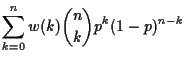
Definition: A statistic ![]() is complete for a model
is complete for a model
![]() if
if
We have already seen that ![]() is complete in the Binomial
is complete in the Binomial![]() model.
In the
model.
In the ![]() model suppose
model suppose

There is only one general tactic. Suppose ![]() has
density
has
density

You prove the sufficiency by the factorization criterion and
the completeness using the properties of Laplace transforms
and the fact that the joint density of
![]()
Example:
![]() model density
has form
model density
has form

Remark: The statistic
![]() is a one to one
function of
is a one to one
function of
![]() so it must be complete
and sufficient, too. Any function of the latter statistic
can be rewritten as a function of the former and vice versa.
so it must be complete
and sufficient, too. Any function of the latter statistic
can be rewritten as a function of the former and vice versa.
FACT: A complete sufficient statistic is also minimal sufficient.
Theorem: If ![]() is a complete sufficient
statistic for some model and
is a complete sufficient
statistic for some model and ![]() is an unbiased
estimate of some parameter
is an unbiased
estimate of some parameter
![]() then
then ![]() is the
UMVUE of
is the
UMVUE of
![]() .
.
Proof: Suppose ![]() is another unbiased estimate
of
is another unbiased estimate
of ![]() . According to Rao-Blackwell,
. According to Rao-Blackwell, ![]() is improved
by
is improved
by ![]() so if
so if ![]() is not UMVUE then there must exist
another function
is not UMVUE then there must exist
another function ![]() which is unbiased and whose variance
is smaller than that of
which is unbiased and whose variance
is smaller than that of ![]() for some value of
for some value of ![]() . But
. But
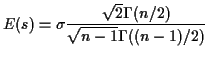
Example: In the
![]() example the random
variable
example the random
variable
![]() has a
has a
![]() distribution.
It follows that
distribution.
It follows that
![$\displaystyle E\left[\frac{\sqrt{n-1}s}{\sigma}\right] =
\frac{\int_0^\infty
x^{1/2} \left(\frac{x}{2}\right)^{(n-1)/2-1} e^{-x/2}
dx}{{2\Gamma((n-1)/2)}}
$](img285.gif)


Binomial![]() log odds is
log odds is
![]() . Since
the expectation of any function of the data is a polynomial function
of
. Since
the expectation of any function of the data is a polynomial function
of ![]() and since
and since ![]() is not a polynomial function of
is not a polynomial function of ![]() there
is no unbiased estimate of
there
is no unbiased estimate of ![]()