We are investigating assumptions on a discrete time process which will permit us to make reasonable estimates of the parameters. We will look for assumptions which guarantee at least the existence
Definition: A stochastic process
![]() is
stationary if the joint distribution of
is
stationary if the joint distribution of
![]() is the same
as the joint distribution of
is the same
as the joint distribution of
![]() for all
for all ![]() and all
and all ![]() .
(Often we call this strictly stationary.)
.
(Often we call this strictly stationary.)
Definition: A stochastic process
![]() is
weakly (or second order) stationary if
is
weakly (or second order) stationary if
Remark:
Definition: ![]() is Gaussian if, for each
is Gaussian if, for each
![]() the vector
the vector
![]() has a Multivariate Normal Distribution.
has a Multivariate Normal Distribution.
Examples of Stationary Processes:
1) Strong Sense White Noise: A process
![]() is strong sense
white noise if
is strong sense
white noise if
![]() is iid with mean 0 and finite variance
is iid with mean 0 and finite variance ![]() .
.
2) Weak Sense White Noise:
![]() is second order stationary with
is second order stationary with

In this course we always use
![]() as notation for white noise and
as notation for white noise and
![]() as the variance of this white noise. We use subscripts to indicate
variances of other things.
as the variance of this white noise. We use subscripts to indicate
variances of other things.
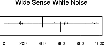
Example Graphics:

2) Moving Averages: if
![]() is white noise then
is white noise then
![]() is stationary. (If you use second order white noise you get second
order stationary. If the white noise is iid you get strict stationarity.)
is stationary. (If you use second order white noise you get second
order stationary. If the white noise is iid you get strict stationarity.)
Example proof:
![]() which is constant as required. Moreover:
which is constant as required. Moreover:

Most of these covariances are 0. For instance

The proof that ![]() is strictly stationary when the
is strictly stationary when the ![]() s are iid is
in your homework; it is quite different.
s are iid is
in your homework; it is quite different.
Example Graphics:
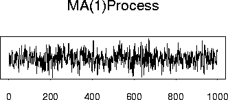
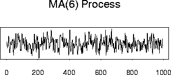
The trajectory of ![]() can be made quite smooth (compared to that of
white noise) by averaging over many
can be made quite smooth (compared to that of
white noise) by averaging over many ![]() s.
s.
3) Autoregressive Processes:
An AR(1) process ![]() is a process satisfying the equations:
is a process satisfying the equations:

Now for
![]() how is
how is ![]() determined from
the
determined from
the
![]() ? (We want to solve the equations
(1) to get an explicit formula for
? (We want to solve the equations
(1) to get an explicit formula for ![]() .)
The case
.)
The case ![]() is notationally simpler. We get
is notationally simpler. We get

Claim: It is a theorem that if ![]() is a weakly stationary
series then
is a weakly stationary
series then
![]() converges (technically
it converges in mean square) and is a second order stationary solution to the
equation (1). If
converges (technically
it converges in mean square) and is a second order stationary solution to the
equation (1). If ![]() is a strictly stationary process then
under some weak assumptions about how heavy the tails of
is a strictly stationary process then
under some weak assumptions about how heavy the tails of ![]() are
are
![]() converges almost surely and is a
strongly stationary solution of (1).
converges almost surely and is a
strongly stationary solution of (1).
In fact if
![]() are constants such that
are constants such that
![]() and
and
![]() is weakly stationary (respectively strongly stationary with finite variance)
then
is weakly stationary (respectively strongly stationary with finite variance)
then

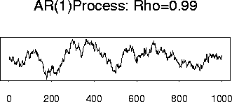
Example Graphics:
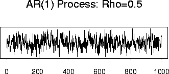
Motivation of the jargon ``filter'' comes from physics. Consider an electric circuit
with a resistance ![]() in series with a capacitance
in series with a capacitance ![]() . We apply an ``input'' voltage
. We apply an ``input'' voltage
![]() across the two elements and measure the voltage drop across the capacitor. We will call
this voltage drop the ``output'' voltage and denote the output
voltage by
across the two elements and measure the voltage drop across the capacitor. We will call
this voltage drop the ``output'' voltage and denote the output
voltage by ![]() . The relevant physical rules are these:
. The relevant physical rules are these:

These rules give


 |
||
 |