STAT 870 Lecture 11
> p:= matrix(2,2,[[3/5,2/5],[1/5,4/5]]);
                      [3/5    2/5]
                 p := [          ]
                      [1/5    4/5]
> p2:=evalm(p*p):
> p4:=evalm(p2*p2):
> p8:=evalm(p4*p4):
> p16:=evalm(p8*p8):
This computes the powers (evalm understands
matrix algebra).
Fact:

> evalf(evalm(p));
            [.6000000000    .4000000000]
            [                          ]
            [.2000000000    .8000000000]
> evalf(evalm(p2));
            [.4400000000    .5600000000]
            [                          ]
            [.2800000000    .7200000000]
> evalf(evalm(p4));
            [.3504000000    .6496000000]
            [                          ]
            [.3248000000    .6752000000]
> evalf(evalm(p8));
            [.3337702400    .6662297600]
            [                          ]
            [.3331148800    .6668851200]
> evalf(evalm(p16));
            [.3333336197    .6666663803]
            [                          ]
            [.3333331902    .6666668098]
Where did 1/3 and 2/3 come from?
Suppose we toss a coin ![]() and start the
chain with Dry if we get heads and Wet if we get
tails.
and start the
chain with Dry if we get heads and Wet if we get
tails.
Then

and

Notice last line is a matrix multiplication of
row vector ![]() by matrix
by matrix ![]() .
A special
.
A special ![]() : if we put
: if we put ![]() and
and ![]() then
then

So: if ![]() then
then ![]() and analogously for W. This means that
and analogously for W. This means that ![]() and
and ![]() have the
same distribution.
have the
same distribution.
A probability vector ![]() is called the initial distribution for
the chain if
is called the initial distribution for
the chain if
![]()
A Markov Chain is stationary if
![]()
for all i
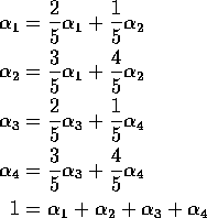
Finding stationary initial distributions. Consider ![]() above. The equation
above. The equation
![]()
is really
![]()
The first can be rearranged to
![]()
and so can the second. If ![]() is to be a
probability vector then
is to be a
probability vector then
![]()
so we get
![]()
leading to
![]()
Some more examples:

Set ![]() and get
and get

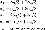
First plus third gives
![]()
so both sums 1/2. Continue algebra to get
![]()
p:=matrix([[0,1/3,0,2/3],[1/3,0,2/3,0],
          [0,2/3,0,1/3],[2/3,0,1/3,0]]);

               [ 0     1/3     0     2/3]
               [                        ]
               [1/3     0     2/3     0 ]
          p := [                        ]
               [ 0     2/3     0     1/3]
               [                        ]
               [2/3     0     1/3     0 ]
> p2:=evalm(p*p);
             [5/9     0     4/9     0 ]
             [                        ]
             [ 0     5/9     0     4/9]
        p2:= [                        ]
             [4/9     0     5/9     0 ]
             [                        ]
             [ 0     4/9     0     5/9]
> p4:=evalm(p2*p2):
> p8:=evalm(p4*p4):
> p16:=evalm(p8*p8):
> p17:=evalm(p8*p8*p):
> evalf(evalm(p16));
    [.5000000116 , 0 , .4999999884 , 0]
    [                                 ]
    [0 , .5000000116 , 0 , .4999999884]
    [                                 ]
    [.4999999884 , 0 , .5000000116 , 0]
    [                                 ]
    [0 , .4999999884 , 0 , .5000000116]
> evalf(evalm(p17));
    [0 , .4999999961 , 0 , .5000000039]
    [                                 ]
    [.4999999961 , 0 , .5000000039 , 0]
    [                                 ]
    [0 , .5000000039 , 0 , .4999999961]
    [                                 ]
    [.5000000039 , 0 , .4999999961 , 0]
> evalf(evalm((p16+p17)/2));
  [.2500, .2500, .2500, .2500]
  [                          ]
  [.2500, .2500, .2500, .2500]
  [                          ]
  [.2500, .2500, .2500, .2500]
  [                          ]
  [.2500, .2500, .2500, .2500]

Solve ![]() :
:

Second and fourth equations redundant. Get

Pick ![]() in [0,1/4];
put
in [0,1/4];
put ![]() .
.
![]()
solves ![]() .
So solution is not unique.
.
So solution is not unique.
> p:=matrix([[2/5,3/5,0,0],[1/5,4/5,0,0],
            [0,0,2/5,3/5],[0,0,1/5,4/5]]);

               [2/5    3/5     0      0 ]
               [                        ]
               [1/5    4/5     0      0 ]
          p := [                        ]
               [ 0      0     2/5    3/5]
               [                        ]
               [ 0      0     1/5    4/5]
> p2:=evalm(p*p):
> p4:=evalm(p2*p2):
> p8:=evalm(p4*p4):
> evalf(evalm(p8*p8));
        [.2500000000 , .7500000000 , 0 , 0]
        [                                 ]
        [.2500000000 , .7500000000 , 0 , 0]
        [                                 ]
        [0 , 0 , .2500000000 , .7500000000]
        [                                 ]
        [0 , 0 , .2500000000 , .7500000000]
Notice that rows converge but to two different vectors:
![]()
and
![]()
Solutions of ![]() revisited?
Check that
revisited?
Check that
![]()
and
![]()
If ![]() (
( ![]() ) then
) then
![]()
so again solution is not unique. Last example:
> p:=matrix([[2/5,3/5,0],[1/5,4/5,0],
             [1/2,0,1/2]]);

                  [2/5    3/5     0 ]
                  [                 ]
             p := [1/5    4/5     0 ]
                  [                 ]
                  [1/2     0     1/2]
> p2:=evalm(p*p):
> p4:=evalm(p2*p2):
> p8:=evalm(p4*p4):
> evalf(evalm(p8*p8));
  [.2500000000 .7500000000        0       ]
  [                                       ]
  [.2500000000 .7500000000        0       ]
  [                                       ]
  [.2500152588 .7499694824 .00001525878906]
Interpretation of examples
![]()
does converge.
Basic distinguishing features: pattern of 0s in matrix ![]() .
.
The ergodic theorem
Consider a finite state space chain.
If x is a vector then the ith entry in ![]() is
is
![]()
Rows of ![]() probability vectors, so a
weighted average of the entries in x.
probability vectors, so a
weighted average of the entries in x.
If the weights are
strictly between 0 and 1 and the largest and smallest entries
in x are not the same then ![]() is strictly
between the largest and smallest entries in x. In fact
is strictly
between the largest and smallest entries in x. In fact
![]()
and
![]()
Now multiply ![]() by
by ![]() .
.
ijth entry in ![]() is a weighted average of the jth
column of
is a weighted average of the jth
column of ![]() .
.
So, if all the entries in row i of ![]() are positive and the jth column of
are positive and the jth column of ![]() is not constant, the
ith entry in the jth column of
is not constant, the
ith entry in the jth column of ![]() must be strictly
between the minimum and maximum entries of the jth column of
must be strictly
between the minimum and maximum entries of the jth column of
![]() .
.
In fact, fix a j.
![]() maximum entry in column j of
maximum entry in column j of ![]()
![]() the minimum
entry.
the minimum
entry.
Suppose all entries of ![]() are positive.
are positive.
Let ![]() be the smallest entry in
be the smallest entry in ![]() . Our argument above
shows that
. Our argument above
shows that
![]()
and
![]()
Putting these together gives
![]()
In summary the column maximum decreases, the column minimum increases
and the gap between the two decreases exponentially along
the sequence ![]() .
.
This idea can be used to prove

Proof: First for k>r
![]()
For each i there is a k for which ![]() and since
and since
![]() we see
we see ![]() .
The argument before the proposition shows that
.
The argument before the proposition shows that
![]()
exists for each m and ![]() . This proves
. This proves ![]() has a limit which
we call
has a limit which
we call ![]() . Since
. Since ![]() also converges to
also converges to ![]() we
find
we
find
![]()
Hence each row of ![]() is a solution of
is a solution of ![]() . The argument
before the statement of the proposition shows all rows of
. The argument
before the statement of the proposition shows all rows of ![]() are equal.
Let
are equal.
Let ![]() be this common row.
be this common row.
Now if ![]() is any vector whose entries sum to 1
then
is any vector whose entries sum to 1
then ![]() converges to
converges to
![]()
If ![]() is any solution of
is any solution of ![]() we have by induction
we have by induction
![]() so
so ![]() so
so ![]() .
That is exactly one vector whose entries sum to 1 satisfies
.
That is exactly one vector whose entries sum to 1 satisfies ![]() .
.
![]()
Note conditions:
There is an r for which all entries in ![]() are positive.
are positive.
The chain has a finite state space.
Consider finite state space case:
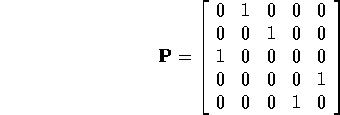
![]() need not have limit. Example:
need not have limit. Example:
![]()
Note ![]() is the identity while
is the identity while ![]() .
Note, too, that
.
Note, too, that
![]()
Consider the equations ![]() with
with ![]() .
We get
.
We get
![]()
so that the solution to ![]() is again unique.
is again unique.
Definition: The period d of a state i is the greatest common divisor of
![]()
![]()
Definition: A state is aperiodic if its period is 1.
Proof: I do the case d=1. Fix i. Let
![]()
If ![]() then
then ![]() .
.
This (and aperiodic) implies (number theory argument) that there is an r such
that ![]() implies
implies ![]() .
.
Now find m and n so that
![]()
For k>r+m+n we see ![]() so the gcd of the
set of k such that
so the gcd of the
set of k such that ![]() is 1.
is 1. ![]()
The case of period d>1 can be dealt with by considering
![]() .
.

For this example ![]() is a class of period 3 states
and
is a class of period 3 states
and ![]() a class of period 2 states.
a class of period 2 states.

has a single communicating class of period 2.
A chain is aperiodic if all its states are aperiodic.