Postscript version of this file

STAT 870 Lecture 12

Hitting Times

Start irreducible recurrent chain in state i. Let be first n;SPMgt;0 such that . Define

First step analysis:

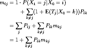
Example

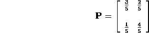
The equations are

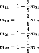
The second and third equations give immediately

Then plug in to the others to get

Notice stationary initial distribution is

Consider fraction of time spent in state j:

Imagine chain starts in chain i; take expected value.

If rows of converge to then fraction converges to ; i.e. limiting fraction of time in state j is .

Heuristic: start chain in i. Expect to return to i every time units. So are in state i about once every time units; i.e. limiting fraction of time in state i is .

Conclusion: for an irreducible recurrent finite state space Markov chain

Real proof: Renewal theorem or variant.

Idea: are times of visits to i. Segment i:

Segments are iid by Strong Markov.

Number of visits to i by time is exactly k.

Total elapsed time is where are iid.

Fraction of time in state i by time is

by SLLN. So if fraction converges to must have

Summary of Theoretical Results:

For an irreducible aperiodic positive recurrent Markov Chain:

1. converges to a stochastic matrix .
2. Each row of is the unique stationary initial distribution.
3. The stationary initial distribution is given by

   

   where is the mean return time to state i from state i.

If the state space is finite an irreducible chain is positive recurrent.

Ergodic Theorem

Notice slight of hand: I showed

but claimed

almost surely which is also true. This is a step in the proof of the ergodic theorem. For an irreducible positive recurrent Markov chain and any f on S such that :

almost surely. The limit works in other senses, too. You also get

E.g.  fraction of transitions from i to j goes to

For an irreducible positive recurrent chain of period d:

1. has d communicating classes each of which forms an irreducible aperiodic positive recurrent chain.
2. has a limit .
3. Each row of is the unique stationary initial distribution.
4. Stationary initial distribution places probability 1/d on each of the communicating classes in 1.

For an irreducible null recurrent chain:

1. converges to 0 (pointwise).
2. there is no stationary initial distribution.

For an irreducible transient chain:

1. converges to 0 (pointwise).
2. there is no stationary initial distribution.

For a chain with more than 1 communicating class:

1. If is a recurrent class the submatrix of made by picking out rows i and columns j for which is a stochastic matrix. The corresponding entries in are just so you can apply the conclusions above.
2. For any transient or null recurrent class the corresponding columns in converge to 0.
3. If there are multiple positive recurrent communicating classes then the stationary initial distribution is not unique.

Poisson Processes

Particles arriving over time at a particle detector. Several ways to describe most common model.

Approach 1: numbers of particles arriving in an interval has Poisson distribution, mean proportional to length of interval, numbers in several non-overlapping intervals independent.

For s;SPMlt;t, denote number of arrivals in (s,t] by N(s,t). Jargon: N(A) = number of points in A is a counting process. Model is

1. N(s,t) has a Poisson distribution.
2. For the variables are independent.

Approach 2:

Let be the times at which the particles arrive.

Let with by convention. are called interarrival times.

Then are independent Exponential random variables with mean .

Note is called survival function of .

Approaches are equivalent. Both are deductions of a model based on local behaviour of process.

Approach 3: Assume:

1. given all the points in [0,t] the probability of 1 point in the interval (t,t+h] is of the form

   

2. given all the points in [0,t] the probability of 2 or more points in interval (t,t+h] is of the form

   

Notation: given functions f and g we write

provided

[Aside: if there is a constant M such that

we say

Notation due to Landau. Another form is

means there is and M s.t. for all

Idea: o(h) is tiny compared to h while O(h) is (very) roughly the same size as h.]

Generalizations:

1. First (Poisson) model generalizes to N(s,t] having a Poisson distribution with parameter for some non-decreasing non-negative function (called cumulative intensity). Result called inhomogeneous Poisson process.
2. Exponential interarrival model generalizes to independent non-exponential interarrival times. Result is renewal process or semi-Markov process.
3. Infinitesimal probability model generalizes to other infinitesimal jump rates. Model specifies infinitesimal generator. Yields other continuous time Markov Chains.