Continuous Probability Distributions

Definitions

Continuous Variable: can take on any value between two specified values. Obtained by measuring.

Discrete Variable: not continuous variable (cannot take on any value between two specified values). Obtained by counting.

Empirical Rules: the statements that tell you approximately what proportion of the values in a data set fall within 1, 2, or 3 standard deviations of the mean.

Exponential Distribution: the probability distribution that describes the time between events in a Poisson process.

Normal Distribution: a distribution with density function 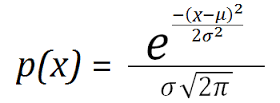. It is bell-shaped and symmetric, and is very common in "real life".

Normal Probability Plot: a quantile-quantile plot where one of the data sets is normally distributed.

Probability Density Function: a function of a continuous random variable, such that the area under the function for an interval gives the probability that the value of the variable lies within the same interval.

Quantile-Quantile Plot: a scatter plot of the quantiles of one data set against the quantiles of another data set.

Rectangular Distribution: see uniform distribution.

Standardized Normal Distribution: (a.k.a. Z-Distribution, a.k.a. Gaussian Distribution, a.k.a. Bell Curve) the normal distribution with mean = 0 and standard deviation = 1.

Standardized Normal Variable: the variable that follows the standardized normal distribution.

Uniform Distribution: (a.k.a. rectangular distribution) a symmetric probability distribution such that a randomly selected value is equally likely to be in every interval of the same length.

Z-Distribution: see Standardized Normal Distribution.

These are the illustrations I have used in class:

The Normal Probability Distribution Graph Interactive from Interactive Mathematics site. Play with it.

The Exponential Distribution Applet, from Matt Bognar's page. Try to enter various values for λ to see how the shape of the binomial distribution depends on this parameter. Entering a value for x will also calculate the probability of the variable being less or equal to that value.

• Try entering λ = 10, then λ = 20, then λ = 100 (without entering x). Do you see anything peculiar about the shape of the distribution?
• Try entering pairs λ = 10 and x = 0.1, then λ = 20 and x = 0.05, then λ = 100 and x = 0.01. Do you see anything peculiar about the calculated P(X<x)?

Notes

It is important to recognize that probability of any given value occuring in a continuous distribution is 0. It is because here we are talking about one value out of infinite number of possible values. For this reason, we cannot build a probability function same way as we did for the discrete variables. Instead, we are using the probability density function which allows us to evaluate probability of a random variable being in a certain interval, not equal to a certain single value.

The normal distribution refers to a family of distributions all looking similar: bell-shaped and symmetrical. Where on the number line you find a normal distribution (its position) is determined by its mean, and how wide the distribution is is determined by its standard deviation. If you know the mean and the standard deviation, you can build a complete density function. In this sense, the two parameters, the mean and the standard deviation, completely describe a normal distribution.

The normal distribution's range is infinity, i.e., a normally distributed valriable may theoretically take on any value.

Transforming any normally distributed variable into a standardized normally distributed variable involves subtracting the mean from every value of the variable and dividing every value by the standard deviation.

The empirical rules (we encountered them several times before) come from a normal distribution.

No data set is ever normally distributed, because the sets have a finite number of values and the normal distribution is continuous. We can, nevertheless, talk about approximately normally distributed data sets.

The exponential distribution is the "inverse" of the Poisson distribution. They describe same process but look at different variables.

Read These

Chapter 6. The Normal Distribution and Other Continuous Distributions in the textbook:

6.1 Continuous Probabilities Distributions (p. 220)

• Try to commit the pictures of the three distributions to your memory.

6.2 The Normal Distribution (pp. 220-231)

• You are not required to memorize the formula for the normal probability density function, but rather know the properties (symmetry and bell shape).
• Determining the probabilities for given values and the values for given probabilities from the Z value table is essential. Make sure you learn how to use the table (doing several exercises that ask to use the table is a very good idea).

6.3 Evaluating Normality (pp. 233-236)

• Understand how to evaluate normality using the theoretical properties of a normal distribution.
• You should be able to build a normal probability plot on your own.

6.4 The Uniform Distribution (pp. 237-239)

6.5 The Exponential Distribution (pp. 240-241)

• Notice that λ in the exponential distribution is the same λ you find in the Poisson distribution if the two of them describe same process.

You may omit sections 6.6 The Normal Approximation to the Binomial Distribution (pp. 242-243)

Watch These

Answer These

File CourseMarks.xlsx has the marks for a course at Taramont University. Use these marks to evaluate the (approximate) normality of the marks distribution:

• by comparing the properties of the data set to the theoretical properties of a normal distribution;
• by constructing a histogram and discussing its shape;
• by constructing a boxplot and discussing its shape;
• by constructing a normal probability plot and discussing its shape.

Assume X is normally distributed with μ = 5 and σ = 2. Use the Z-table to find:

• P(X<8);
• P(X>6);
• P(3<X<6);
• A such that P(X<A) = 0.6;
• B such that P(X>B) = 0.2;

Wikipedia says that Cristiano_Ronaldo has scored 423 goals in 620 games. Using the exponential distribution, find the probability that he will score a goal in the next game (against Austria, on Saturday, June 18).

Using the Poisson distribution, find the probability that he will score a goal in the next game (against Austria, on Saturday, June 18). Hint: you must get same answer as in the previous problem (with the exponential distribution).