Chapter Contents
Previous
Next
|
Chapter Contents |
Previous |
Next |
| The MODEL Procedure |
PROC MODEL currently supports two methods for minimizing the objective function. These methods are described in the following sections.
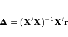
where ![]() is the change vector,
X is the stacked ng ×p Jacobian
matrix of partial derivatives of the residuals with
respect to the parameters, and r is an ng ×1vector of the stacked residuals.
The components of X and r are weighted by the S-1 matrix.
When instrumental methods are used, X and r are the projections
of the Jacobian matrix and residuals vector in the instruments space
and not the Jacobian and residuals themselves.
In the preceding formula, S and W are suppressed. If instrumental variables
are used, then the change vector becomes:
is the change vector,
X is the stacked ng ×p Jacobian
matrix of partial derivatives of the residuals with
respect to the parameters, and r is an ng ×1vector of the stacked residuals.
The components of X and r are weighted by the S-1 matrix.
When instrumental methods are used, X and r are the projections
of the Jacobian matrix and residuals vector in the instruments space
and not the Jacobian and residuals themselves.
In the preceding formula, S and W are suppressed. If instrumental variables
are used, then the change vector becomes:

This vector is computed at the end of each iteration.
The objective function is then computed at the changed parameter values at the
start of the next iteration.
If the objective function is not improved by the change,
the ![]() vector is reduced by one-half and the objective function
is re-evaluated.
The change vector will be halved up to MAXSUBITER= times until
the objective function is improved.
For FIML the X'X matrix is substituted with
one of three choices for approximations to the Hessian. See the
"FIML Estimation" section in this chapter.
vector is reduced by one-half and the objective function
is re-evaluated.
The change vector will be halved up to MAXSUBITER= times until
the objective function is improved.
For FIML the X'X matrix is substituted with
one of three choices for approximations to the Hessian. See the
"FIML Estimation" section in this chapter.
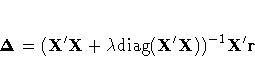
where ![]() is the change vector, and X and r are the same
as for the Gauss-Newton method, described in the preceding section.
Before the iterations start,
is the change vector, and X and r are the same
as for the Gauss-Newton method, described in the preceding section.
Before the iterations start, ![]() is set to a small value (1E-6).
At each iteration,
the objective function is evaluated at the parameters changed by
is set to a small value (1E-6).
At each iteration,
the objective function is evaluated at the parameters changed by ![]() .
If the objective function is not improved,
.
If the objective function is not improved,
![]() is increased to 10
is increased to 10![]() and the step is tried again.
and the step is tried again.
![]() can be increased up to MAXSUBITER= times
to a maximum of 1E15 (whichever comes first) until the objective
function is improved.
For the start of the next iteration,
can be increased up to MAXSUBITER= times
to a maximum of 1E15 (whichever comes first) until the objective
function is improved.
For the start of the next iteration, ![]() is reduced to
max(
is reduced to
max(![]() /10,1E-10).
/10,1E-10).
|
Chapter Contents |
Previous |
Next |
Top |
Copyright © 1999 by SAS Institute Inc., Cary, NC, USA. All rights reserved.