Chapter Contents
Previous
Next
|
Chapter Contents |
Previous |
Next |
| The STATESPACE Procedure |
After computing the sample autocovariance matrices, PROC STATESPACE fits a sequence of vector autoregressive models. These preliminary autoregressive models are used to estimate the autoregressive order of the process and limit the order of the autocovariances considered in the state vector selection process.
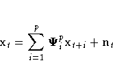
Let xt be the r-component stationary time series given by the VAR statement after differencing and subtracting the vector of sample means. (If the NOCENTER option is specified, the mean is not subtracted.) Let n be the number of observations of xt from the input data set.
Let et be a vector white noise sequence
with mean vector 0 and variance matrix ![]() , and
let nt be a vector white noise sequence with
mean vector 0 and variance matrix
, and
let nt be a vector white noise sequence with
mean vector 0 and variance matrix ![]() .Let p be the order of the vector autoregressive model
for xt.
.Let p be the order of the vector autoregressive model
for xt.
The forward autoregressive form based on the past observations is written as follows:

The backward autoregressive form based on the future observations is written as follows:
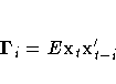
Letting E denote the expected value operator,
the autocovariance sequence for the xt series,
![]() , is
, is
The Yule-Walker equations for the autoregressive model that matches the first p elements of the autocovariance sequence are
![[\matrix{
{\Gamma}_{0} & {\Gamma}_{1} & { ... } & {\Gamma}_{p-1} \cr
{\Gamma}^...
...
[\matrix{
{\Gamma}_{1} \cr
{\Gamma}_{2} \cr
{\vdots} \cr
{\Gamma}_{p}
} ]](images/staeq19.gif)
and
![[\matrix{
{\Gamma}_{0} &
{\Gamma}'_{1} &
{ ... } & {\Gamma}'_{p-1} \cr
{\Gam...
...matrix{
{\Gamma}_{1}' \cr
{\Gamma}_{2}' \cr
{\vdots} \cr
{\Gamma}_{p}'
} ]](images/staeq20.gif)
Here ![]() are the coefficient
matrices for the past observation form of the vector autoregressive model,
and
are the coefficient
matrices for the past observation form of the vector autoregressive model,
and ![]() are the coefficient
matrices for the future observation form.
More information on the Yule-Walker equations in the multivariate
setting can be found in Whittle (1963) and Ansley and Newbold (1979).
are the coefficient
matrices for the future observation form.
More information on the Yule-Walker equations in the multivariate
setting can be found in Whittle (1963) and Ansley and Newbold (1979).
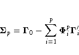
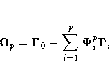
The innovation variance matrices for the two forms can be written as follows:
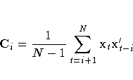
The autoregressive models are fit to the data using the preceding
Yule-Walker equations with ![]() replaced by the
sample covariance sequence Ci.
The covariance matrices are calculated as
replaced by the
sample covariance sequence Ci.
The covariance matrices are calculated as
Let ![]() ,
, ![]() ,
,![]() , and
, and ![]() represent the Yule-Walker estimates of
represent the Yule-Walker estimates of ![]() ,
,![]() ,
, ![]() , and
, and
![]() respectively.
These matrices are written to an output data set when the OUTAR=
option is specified.
respectively.
These matrices are written to an output data set when the OUTAR=
option is specified.
When the PRINTOUT=LONG option is specified,
the sequence of matrices ![]() and the corresponding correlation matrices are printed.
The sequence of matrices
and the corresponding correlation matrices are printed.
The sequence of matrices ![]() is used to compute Akaike information criteria
for selection of the autoregressive order of the process.
is used to compute Akaike information criteria
for selection of the autoregressive order of the process.
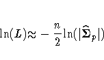
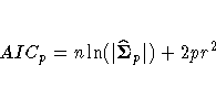
Thus, the AIC for the order p model is computed as
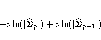
You can use the printed AIC array to compute a likelihood ratio test of the autoregressive order. The log-likelihood ratio test statistic for testing the order p model against the order p-1 model is
This quantity is asymptotically distributed as a
![]() with r2 degrees of freedom if
the series is autoregressive of order p-1.
It can be computed from the AIC array as
with r2 degrees of freedom if
the series is autoregressive of order p-1.
It can be computed from the AIC array as
You can evaluate the significance of these test statistics with
the PROBCHI function in a SAS DATA step, or with a ![]() table.
table.
By default, PROC STATESPACE selects the order, p, producing the autoregressive model with the smallest AICp. If the value p for the minimum AICp is less than the value of the PASTMIN= option, then p is set to the PASTMIN= value. Alternatively, you can use the ARMAX= and PASTMIN= options to force PROC STATESPACE to use an order you select.
The partial autocorrelations are from
the sample partial autoregressive matrices
![]() .The standard errors used for the significance limits
of the partial autocorrelations are
computed from the sequence of matrices
.The standard errors used for the significance limits
of the partial autocorrelations are
computed from the sequence of matrices
![]() and
and ![]() .
.
Under the assumption that the observed series arises from an
autoregressive process of order p-1,
the pth sample partial autoregressive matrix
![]() has an asymptotic variance matrix
has an asymptotic variance matrix
![]() .
.
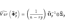
The significance limits for ![]() used in the schematic plot of the sample partial autoregressive sequence
are derived by replacing
used in the schematic plot of the sample partial autoregressive sequence
are derived by replacing ![]() and
and ![]() with their sample estimators to produce the variance estimate,
as follows:
with their sample estimators to produce the variance estimate,
as follows:
|
Chapter Contents |
Previous |
Next |
Top |
Copyright © 1999 by SAS Institute Inc., Cary, NC, USA. All rights reserved.