Introductory Examples
The following introductory examples illustrate how to get started
using the NLP procedure.
An Unconstrained Problem
Consider the simple example of minimizing the
Rosenbrock function (Rosenbrock 1960).
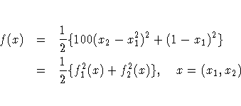
The minimum function value is f(x*) = 0 at x* = (1,1).
This problem does not have any constraints.
The following statements can be used to solve this problem:
   proc nlp;
      min f;
      decvar x1 x2;
      f1 = 10 * (x2 - x1 * x1);
      f2 = 1 - x1;
      f  = .5 * (f1 * f1 + f2 * f2);
   run;
The MIN statement identifies the symbol f that characterizes
the objective function in terms of f1 and f2, and the
DECVAR statement names the decision variables X1 and X2.
Because there is no explicit optimizing algorithm option specified (TECH=)
PROC NLP uses the Newton-Raphson method with ridging,
the default algorithm when there are no constraints.
A better way to solve this problem is to take advantage of the fact
that f is a sum of squares of f1 and f2 and to treat it as a
least-squares problem.
Using the LSQ statement instead of the MIN statement tells
the procedure that this is a least-squares problem, which results
in the use of
one of the specialized algorithms for solving least-squares
problems (for example Levenberg-Marquardt).
   proc nlp;
      lsq f1 f2;
      decvar x1 x2;
      f1 = 10 * (x2 - x1 * x1);
      f2 = 1 - x1;
   run;
The LSQ statement results in the minimization of a function
that is the sum of squares of functions that appear in the LSQ
statement. The least-squares specification is
preferred because it enabless the procedure to exploit the
structure in the problem for numeric stability and performance.
|
| PROC NLP: Least Squares Minimization |
| Parameter Estimates |
2 |
| Functions (Observations) |
2 |
| Optimization Start |
| Active Constraints |
0 |
Objective Function |
3.25 |
| Max Abs Gradient Element |
25.5 |
Radius |
358.01571195 |
| Iteration |
|
Restarts |
Function
Calls |
Active
Constraints |
|
Objective
Function |
Objective
Function
Change |
Max Abs
Gradient
Element |
Lambda |
Ratio
Between
Actual
and
Predicted
Change |
| 1 |
|
0 |
2 |
0 |
|
3.12500 |
0.1250 |
50.0000 |
0 |
0.0385 |
| 2 |
|
0 |
3 |
0 |
|
3.6214E-29 |
3.1250 |
3.62E-14 |
0 |
1.000 |
| Optimization Results |
| Iterations |
2 |
Function Calls |
4 |
| Jacobian Calls |
3 |
Active Constraints |
0 |
| Objective Function |
3.621365E-29 |
Max Abs Gradient Element |
3.619327E-14 |
| Lambda |
0 |
Actual Over Pred Change |
1 |
| Radius |
5 |
|
|
| ABSGCONV convergence criterion satisfied. |
| PROC NLP: Least Squares Minimization |
| Optimization Results |
| Parameter Estimates |
| N |
Parameter |
Estimate |
Gradient
Objective
Function |
| 1 |
x1 |
1.000000 |
-3.61933E-14 |
| 2 |
x2 |
1.000000 |
2.220446E-14 |
|
Figure 5.1: Least-Squares Minimization
PROC NLP displays the iteration history and the solution to this
least-squares problem as shown in Figure 5.1.
It shows that the solution has x1=1 and x2=1.
As expected in an unconstrained problem,
the gradient at the solution is very close to 0.
Boundary Constraints on the Decision Variables
Bounds on the decision variables can be used.
Suppose, for example, that it is necessary to constrain the
decision variables in the previous example to be less than 0.5.
That can be done by adding a BOUNDS statement.
   proc nlp;
      lsq f1 f2;
      decvar x1 x2;
      bounds x1 - x2 <= .5;
      f1 = 10 * (x2 - x1 * x1);
      f2 = 1 - x1;
   run;
The solution in Figure 5.2 shows that the decision variables
meet the constraint bounds.
|
| PROC NLP: Least Squares Minimization |
| Optimization Results |
| Parameter Estimates |
| N |
Parameter |
Estimate |
Gradient
Objective
Function |
Active
Bound
Constraint |
| 1 |
x1 |
0.500000 |
-0.500000 |
Upper BC |
| 2 |
x2 |
0.250000 |
0 |
|
|
Figure 5.2: Least-Squares with Bounds Solution
Linear Constraints on the Decision Variables
More general linear equality or inequality constraints
of the form
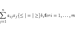
can be specified in a LINCON statement.
For example, suppose that in addition to the bounds constraints
on the decision variables it is necessary to guarantee that the
sum x1 + x2 is less than or equal to 0.6.
That can be achieved by adding a LINCON statement:
   proc nlp;
      lsq f1 f2;
      decvar x1 x2;
      bounds x1 - x2 <= .5;
      lincon x1 + x2 <= .6;
      f1 = 10 * (x2 - x1 * x1);
      f2 = 1 - x1;
   run;
The output in Figure 5.3 displays the iteration history and
the convergence criterion.
|
| PROC NLP: Least Squares Minimization |
| Gradient is computed using analytic formulas. |
| Cross product Jacobian is computed using analytic formulas. |
| NOTE: |
Initial point was changed to be feasible for boundary and linear constraints. |
|
| PROC NLP: Least Squares Minimization |
| Value of Objective Function = 29.25 |
| PROC NLP: Least Squares Minimization |
| Levenberg-Marquardt Optimization |
| Scaling Update of More (1978) |
| Parameter Estimates |
2 |
| Functions (Observations) |
2 |
| Lower Bounds |
0 |
| Upper Bounds |
2 |
| Linear Constraints |
1 |
| Iteration |
|
Restarts |
Function
Calls |
Active
Constraints |
|
Objective
Function |
Objective
Function
Change |
Max Abs
Gradient
Element |
Lambda |
Ratio
Between
Actual
and
Predicted
Change |
| 1 |
|
0 |
3 |
0 |
|
8.19877 |
21.0512 |
39.5420 |
0.0170 |
0.729 |
| 2 |
|
0 |
4 |
0 |
|
1.05752 |
7.1412 |
13.6170 |
0.0105 |
0.885 |
| 3 |
|
0 |
5 |
1 |
|
1.04396 |
0.0136 |
18.6337 |
0 |
0.0128 |
| 4 |
|
0 |
6 |
1 |
|
0.16747 |
0.8765 |
0.5552 |
0 |
0.997 |
| 5 |
|
0 |
7 |
1 |
|
0.16658 |
0.000895 |
0.000324 |
0 |
0.998 |
| 6 |
|
0 |
8 |
1 |
|
0.16658 |
3.06E-10 |
5.911E-7 |
0 |
0.998 |
| Optimization Results |
| Iterations |
6 |
Function Calls |
9 |
| Jacobian Calls |
7 |
Active Constraints |
1 |
| Objective Function |
0.1665792899 |
Max Abs Gradient Element |
5.9108825E-7 |
| Lambda |
0 |
Actual Over Pred Change |
0.998176801 |
| Radius |
0.0000532357 |
|
|
| GCONV convergence criterion satisfied. |
| PROC NLP: Least Squares Minimization |
| Value of Objective Function = 0.1665792899 |
|
Figure 5.3: Least-Squares with Bounds and Linear Constraints Iteration History
Figure 5.4 shows that the solution
satisfies the linear constraint.
Note that the procedure displays the
active constraints (the constraints that are tight) at optimality.
|
| PROC NLP: Least Squares Minimization |
| Optimization Results |
| Parameter Estimates |
| N |
Parameter |
Estimate |
Gradient
Objective
Function |
| 1 |
x1 |
0.423645 |
-0.312000 |
| 2 |
x2 |
0.176355 |
-0.312001 |
| Linear Constraints Evaluated at Solution |
| 1 |
ACT |
-2.776E-17 |
= |
0.6000 |
- |
1.0000 |
* |
x1 |
- |
1.0000 |
* |
x2 |
|
Figure 5.4: Least-Squares with Bounds and Linear Constraints Solution
Nonlinear Constraints on the Decision Variables
More general nonlinear equality or inequality constraints
can be specified using an NLINCON statement.
Consider the least-squares problem with the additional
constraint

This constraint is specified by a new function c1 constrained
to be greater than or equal to 0 in the NLINCON statement.
The function c1 is defined in the programming statements.
   proc nlp tech=QUANEW;
      min f;
      decvar x1 x2;
      bounds x1 - x2 <= .5;
      lincon x1 + x2 <= .6;
      nlincon c1 >= 0;

      c1 = x1 * x1 - 2 * x2;

      f1 = 10 * (x2 - x1 * x1);
      f2 = 1 - x1;

      f = .5 * (f1 * f1 + f2 * f2);
   run;
Not all of the optimization methods support
nonlinear constraints.
In particular the Levenberg-Marquardt method, the default
for LSQ, does not support nonlinear constraints.
(For more information about the particular algorithms, see the section "Optimization Algorithms".)
The Quasi-Newton method is the prime choice for solving
nonlinear programs with nonlinear constraints.
The option TECH=QUANEW in the PROC NLP statement
causes the Quasi-Newton method to be used.
Figure 5.5 shows the iteration history.
|
| PROC NLP: Nonlinear Minimization |
| Parameter Estimates |
2 |
| Lower Bounds |
0 |
| Upper Bounds |
2 |
| Linear Constraints |
1 |
| Nonlinear Constraints |
1 |
| Optimization Start |
| Objective Function |
5.6880375034 |
Maximum Constraint Violation |
0 |
| Maximum Gradient of the Lagran Func |
33.006897503 |
|
|
| Iteration |
|
Restarts |
Function
Calls |
Objective
Function |
Maximum
Constraint
Violation |
Predicted
Function
Reduction |
Step
Size |
Maximum
Gradient
Element
of the
Lagrange
Function |
| 1 |
|
0 |
12 |
0.72525 |
0 |
0.4043 |
0.831 |
7.728 |
| 2 |
|
0 |
13 |
0.45832 |
0 |
0.0748 |
1.000 |
2.095 |
| 3 |
|
0 |
14 |
0.41405 |
0 |
0.0164 |
1.000 |
0.934 |
| 4 |
' |
0 |
15 |
0.39828 |
0 |
0.1557 |
1.000 |
1.948 |
| 5 |
* |
0 |
16 |
0.44009 |
0 |
0.3277 |
1.000 |
2.802 |
| 6 |
|
0 |
17 |
0.37522 |
0 |
0.0629 |
1.000 |
0.445 |
| 7 |
|
0 |
18 |
0.33828 |
0 |
0.0182 |
1.000 |
0.879 |
| 8 |
|
0 |
19 |
0.33291 |
0 |
0.00592 |
1.000 |
0.322 |
| 9 |
|
0 |
20 |
0.33018 |
0 |
0.000300 |
1.000 |
0.0440 |
| 10 |
|
0 |
21 |
0.33004 |
0 |
0.000016 |
1.000 |
0.00536 |
| 11 |
|
0 |
22 |
0.33003 |
0 |
1.573E-7 |
1.000 |
0.00009 |
| Optimization Results |
| Iterations |
11 |
Function Calls |
23 |
| Gradient Calls |
14 |
Active Constraints |
0 |
| Objective Function |
0.3300307942 |
Maximum Constraint Violation |
0 |
| Maximum Projected Gradient |
3.049416688 |
Value Lagrange Function |
0.3300307942 |
| Maximum Gradient of the Lagran Func |
3.049416688 |
Slope of Search Direction |
-1.572951E-7 |
|
Figure 5.5: Least-Squares with Bounds, Linear and Nonlinear Constraints, Iteration History
Figure 5.6 shows the solution to this problem.
|
| PROC NLP: Nonlinear Minimization |
| Optimization Results |
| Parameter Estimates |
| N |
Parameter |
Estimate |
Gradient
Objective
Function |
Gradient
Lagrange
Function |
| 1 |
x1 |
0.246929 |
0.752559 |
0.752559 |
| 2 |
x2 |
0.030487 |
-3.048708 |
-3.048708 |
| Linear Constraints Evaluated at Solution |
| 1 |
|
0.32258 |
= |
0.6000 |
- |
1.0000 |
* |
x1 |
- |
1.0000 |
* |
x2 |
| Values of Nonlinear Constraints |
| Constraint |
Value |
Residual |
Lagrange
Multiplier |
|
| [ |
2 |
] |
c1_G |
2.06E-7 |
2.06E-7 |
. |
|
|
Figure 5.6: Least-Squares with Bounds, Linear and Nonlinear Constraints, Solution
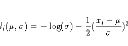
A Simple Maximum Likelihood Example
The following is a very simple example of a maximum likelihood
estimation problem with the log likelihood function:
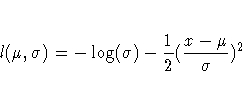
The maximum likelihood estimates of the parameters  and
and  is the solution to
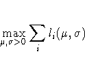
where
In the following DATA step, values for x are input into SAS data set X;
this data set provides the values of xi.
    data x;
      input x @@;
    datalines;
    1 3 4 5 7
    ;
In the following statements, the DATA=X specification drives the
building of the objective function.
When each observation in the DATA=X data set is read,
a new term  using the value of xi
is added to the objective function LOGLIK specified in the
MAX statement.
using the value of xi
is added to the objective function LOGLIK specified in the
MAX statement.
    proc nlp data=x vardef=n covariance=h pcov phes;
      profile mean sigma / alpha=.5 .1 .05 .01;
      max loglik;
      parms mean=0, sigma=1;
      bounds sigma > 1e-12;
      loglik=-0.5*((x-mean)/sigma)**2-log(sigma);
   run;
After a few iterations of the default Newton-Raphson optimization
algorithm, PROC NLP procedure produces the following results.
Figure 5.7: Maximum Likelihood Estimates
In unconstrained maximization, the gradient (that is, the vector of
first derivatives) at the solution must be very close to zero
and the Hessian matrix at the solution
(that is, the matrix of second derivatives) must have
nonpositive eigenvalues.
|
| PROC NLP: Nonlinear Maximization |
| Hessian Matrix |
| |
mean |
sigma |
| mean |
-1.250000003 |
1.33149E-10 |
| sigma |
1.33149E-10 |
-2.500000014 |
|
Figure 5.8: Hessian Matrix
Under reasonable assumptions, the approximate standard errors
of the estimates are the square roots of the
diagonal elements of the covariance matrix of the
parameter estimates which (because of the COV=H specification)
is the same as the inverse of the Hessian matrix:
|
| PROC NLP: Nonlinear Maximization |
Covariance Matrix 2: H = (NOBS/d)
inv(G) |
| |
mean |
sigma |
| mean |
0.7999999982 |
4.260769E-11 |
| sigma |
4.260769E-11 |
0.3999999978 |
|
Figure 5.9: Covariance Matrix
The PROFILE statement computes the values of
the profile likelihood confidence limits on SIGMA and the MEAN
as specified.
|
| PROC NLP: Nonlinear Maximization |
| Wald and PL Confidence Limits |
| N |
Parameter |
Estimate |
Alpha |
Profile Likelihood Confidence
Limits |
Wald Confidence Limits |
| 1 |
mean |
4.000000 |
0.500000 |
3.384431 |
4.615569 |
3.396718 |
4.603282 |
| 1 |
mean |
. |
0.100000 |
2.305716 |
5.694284 |
2.528798 |
5.471202 |
| 1 |
mean |
. |
0.050000 |
1.849538 |
6.150462 |
2.246955 |
5.753045 |
| 1 |
mean |
. |
0.010000 |
0.670351 |
7.329649 |
1.696108 |
6.303892 |
| 2 |
sigma |
2.000000 |
0.500000 |
1.638972 |
2.516078 |
1.573415 |
2.426585 |
| 2 |
sigma |
. |
0.100000 |
1.283506 |
3.748633 |
0.959703 |
3.040297 |
| 2 |
sigma |
. |
0.050000 |
1.195936 |
4.358321 |
0.760410 |
3.239590 |
| 2 |
sigma |
. |
0.010000 |
1.052584 |
6.064107 |
0.370903 |
3.629097 |
|
Figure 5.10: Confidence Limits
Copyright © 1999 by SAS Institute Inc., Cary, NC, USA. All rights reserved.