Statistics
Finally, the transaction
flows to a Bucket, which collects
transactions and can also save the value of transaction attributes
in a SAS data set.
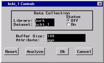
Figure 1.7: A Bucket Control Panel
From the bucket control panel (Figure 1.7)
you can set the size of the
transaction collection buffer and name the transaction attribute
to accumulate.
You can also name a SAS data set into which to collect the
transaction attribute values.
|
| Distribution Function Estimate |
| The UNIVARIATE Procedure |
| Variable: value |
| Moments |
| N |
1803 |
Sum Weights |
1803 |
| Mean |
24.5093328 |
Sum Observations |
44190.3271 |
| Std Deviation |
14.8024337 |
Variance |
219.112044 |
| Skewness |
-0.1060516 |
Kurtosis |
-1.2191446 |
| Uncorrected SS |
1477915.34 |
Corrected SS |
394839.903 |
| Coeff Variation |
60.3950903 |
Std Error Mean |
0.34860632 |
| Basic Statistical Measures |
| Location |
Variability |
| Mean |
24.50933 |
Std Deviation |
14.80243 |
| Median |
26.21585 |
Variance |
219.11204 |
| Mode |
. |
Range |
53.62360 |
| |
|
Interquartile Range |
26.10309 |
| Tests for Location: Mu0=0 |
| Test |
Statistic |
p Value |
| Student's t |
t |
70.30662 |
Pr > |t| |
<.0001 |
| Sign |
M |
901.5 |
Pr >= |M| |
<.0001 |
| Signed Rank |
S |
813153 |
Pr >= |S| |
<.0001 |
| Quantiles (Definition 5) |
| Quantile |
Estimate |
| 100% Max |
53.62741148 |
| 99% |
50.95981599 |
| 95% |
46.44804080 |
| 90% |
43.36915659 |
| 75% Q3 |
37.45295397 |
| 50% Median |
26.21585009 |
| 25% Q1 |
11.34985903 |
| 10% |
3.08194661 |
| 5% |
1.38985610 |
| 1% |
0.28776996 |
| 0% Min |
0.00381383 |
| Extreme Observations |
| Lowest |
Highest |
| Value |
Obs |
Value |
Obs |
| 0.00381383 |
1442 |
51.9481 |
819 |
| 0.02449773 |
1486 |
52.1543 |
818 |
| 0.02846473 |
1458 |
52.1938 |
418 |
| 0.04001101 |
1249 |
52.4247 |
419 |
| 0.06573967 |
1700 |
53.6274 |
817 |
|
Figure 1.8: Statistics on a Transaction Attribute
If you collect data into a SAS data set and then
press the Analyze button,
univariate statistics will be calculated
by the UNIVARIATE procedure (Figure 1.8)
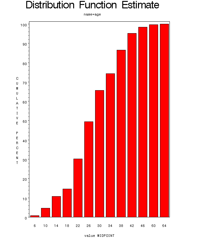
and a sample distribution function
as shown in Figure 1.9
will be plotted.
Figure 1.9: Sample Distribution Function
See Chapter 8, "Analyzing the Sample Path," for more information on
on collecting statistics and analyzing simulation data.
Copyright © 1999 by SAS Institute Inc., Cary, NC, USA. All rights reserved.

