Queue Length

Analyzing the Sample Path

Queue Length

The QSIM Application will generate and execute SAS code that calculates summary statistics on the length of a queue. When you want to start collecting the sample data, you select the On radio button in the Simulation control panel. This starts data collection. When you are ready to generate sample statistics select the component for which you want the statistics and then click the Analyze button. For example, you display data on the queue length on the single-queue multiple-server model in Figure 8.1 by selecting FIFOQueue 1 in the Simulation Control panel and then by pressing Analyze.

Figure 8.4: Statistics on Queue Length

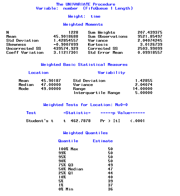
This generates the report shown in Figure 8.4 in the SAS Output Window. Figure 8.4 shows that the sample mean queue length is approximately 45.90 and that the sample variance is approximately 2.04.

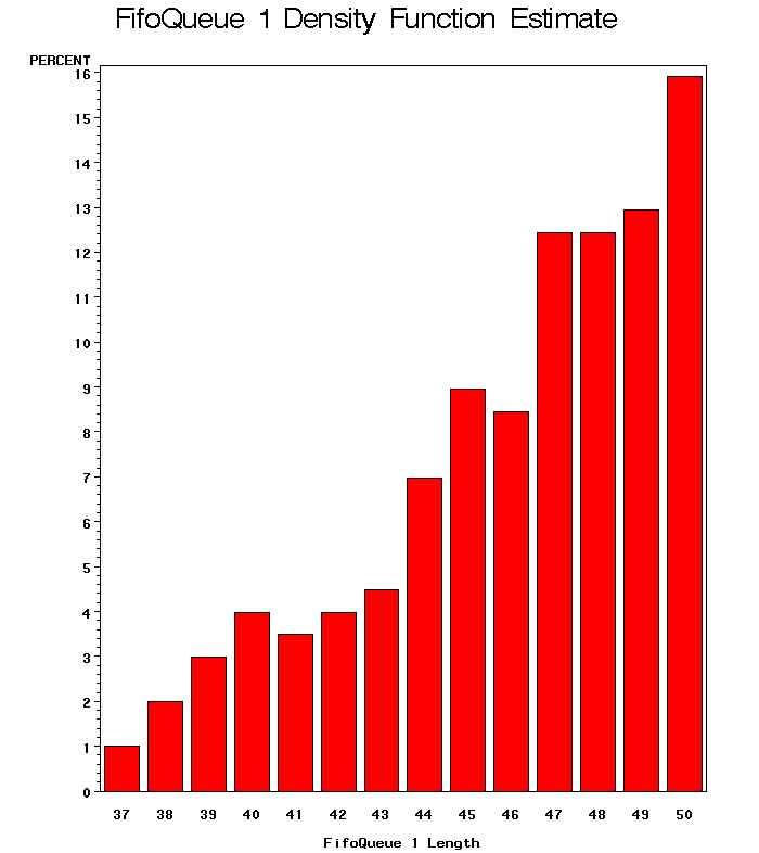
The Analyze button also opens a graphics window with the histogram on the queue length as shown in Figure 8.5. This shows the sample distribution of queue length for the complete sample path that was collected from the time the Collect Data check box is selected until the time the Analyze button is selected.

Figure 8.5: Queue Length Histogram

It is important to note that the observations in the sample path are not independent. There can be a significant amount of autocorrelation in the observations of queue length.

Another way to get Queue Length Statistics

Another way you can obtain statistics on queue length and server utilization is by using the chart components. You take the queue that you want to monitor and drag it into one of the chart components, the VHistogram for example. When you drop the queue, a control panel will open from which you can select the attribute of the component that you want sampled and the distribution to control sampling. Figure 8.6 shows an example. Here the size is selected to be monitored, and the component is to be sampled with a deterministic inter-sample time of one time unit. This is the default sampling distribution. This is different than using the Simulation control panel because in that case all state changes are captured, when using a chart component the queue state is sampled.

Figure 8.6: Sample Component State Control Panel

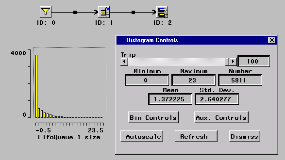
This control panel is opened when the queue labeled "ID: 1" in Figure 2.17 is dropped on the histogram.

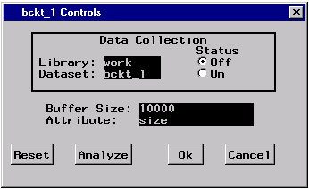
Figure 8.7: Vertical Histogram of the FIFO Queue length

Figure 2.17 also shows the histogram control panel opened. Notice that the control panel shows the simple statistics: minimum, maximum, mean, and standard deviation. Also note that when a component is dropped on a chart, a bucket is automatically associated with the chart component. The bucket is where the sample is collected. The controls for this implicit bucket can be viewed by clicking the Bin Controls button in the Histogram Controls window. it opens the control panel for the bucket as shown in Figure 2.15.

Figure 8.8: Bucket Control Panel

You can display more detailed statistics on queue length using SAS data sets. The "Data Collection" section in the Bucket control panel shows a data collection Status check box. If this is selected, then data on the component state changes are routed to the SAS data set named WORK.BCKT_1. If sample data have been collected for a time, then clicking the Analyze button will generate a univariate analysis performed by the UNIVARIATE procedure and a histogram.

Chapter Contents
Previous
Next
Top