Chi-Square Tests and Statistics

The FREQ Procedure

Chi-Square Tests and Statistics

When you specify the CHISQ option in the TABLES statement, PROC FREQ performs the following chi-square tests for each two-way table: Pearson chi-square, continuity-adjusted chi-square for 2 ×2 tables, likelihood-ratio chi-square, Mantel-Haenszel chi-square, and Fisher's exact test for 2 ×2 tables. Also, PROC FREQ computes the following statistics derived from the Pearson chi-square: the phi coefficient, the contingency coefficient, and Cramer's V. PROC FREQ computes Fisher's exact test for general R ×C tables when you specify the FISHER (or EXACT) option in the TABLES statement, or, equivalently, when you specify the FISHER option in the EXACT statement.

For one-way frequency tables, PROC FREQ performs a chi-square goodness-of-fit test when you specify the CHISQ option. The other chi-square tests and statistics described in this section are defined only for two-way tables and so are not computed for one-way frequency tables.

All the two-way test statistics described in this section test the null hypothesis of no association between the row variable and the column variable. When the sample size n is large, these test statistics are distributed approximately as chi-square when the null hypothesis is true. When the sample size is not large, exact tests may be useful. PROC FREQ computes exact tests for the following chi-square statistics when you specify the corresponding option in the EXACT statement: Pearson chi-square, likelihood-ratio chi-square, and Mantel-Haenszel chi-square. See the section "Exact Statistics" for more information.

Note that the Mantel-Haenszel chi-square statistic is appropriate only when both variables lie on an ordinal scale. The other chi-square tests and statistics in this section are appropriate for either nominal or ordinal variables. The following sections give the formulas that PROC FREQ uses to compute the chi-square tests and statistics. For further information on the formulas and on the applicability of each statistic, refer to Agresti (1996), Stokes, Davis, and Koch (1995), and the other references cited for each statistic.

Chi-Square Test for One-Way Tables

For one-way frequency tables, the CHISQ option in the TABLES statement computes a chi-square goodness-of-fit test. Let C denote the number of classes, or levels, in the one-way table. Let f_i denote the frequency of class i (or the number of observations in class i) for i = 1,2,...,C. Then PROC FREQ computes the chi-square statistic as

$Q_{P} = \sum_{i=1}^C \frac{( f_{i} - e_{i})^2} {e_{i}}$

where e_i is the expected frequency for class i under the null hypothesis.

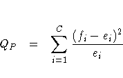
In the test for equal proportions, which is the default for the CHISQ option, the null hypothesis specifies equal proportions of the total sample size for each class. Under this null hypothesis, the expected frequency for each class equals the total sample size divided by the number of classes,

$e_{i} = n / C { for } i = 1,2, ... ,C$

In the test for specified frequencies, which PROC FREQ computes when you input null hypothesis frequencies using the TESTF= option, the expected frequencies are those TESTF= values. In the test for specified proportions, which PROC FREQ computes when you input null hypothesis proportions using the TESTP= option, the expected frequencies are determined from the TESTP= proportions p_i, as

$e_{i} = p_{i} \cdot n { for } i = 1,2, ... ,C$

Under the null hypothesis (of equal proportions, specified frequencies, or specified proportions), this test statistic has an asymptotic chi-square distribution, with C - 1 degrees of freedom. In addition to the asymptotic test, PROC FREQ computes the exact one-way chi-square test when you specify the CHISQ option in the EXACT statement.

Chi-Square Test for Two-Way Tables

The Pearson chi-square statistic for two-way tables involves the differences between the observed and expected frequencies, where the expected frequencies are computed under the null hypothesis of independence. The chi-square statistic is computed as

$Q_P = \sum_i \sum_j \frac{(n_{ij} - e_{ij})^2}{e_{ij}}$

where

e_ij = [(n_{i ·} n_·j)/n]

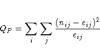
When the row and column variables are independent, Q_P has an asymptotic chi-square distribution with (R-1)(C-1) degrees of freedom. For large values of Q_P, this test rejects the null hypothesis in favor of the alternative hypothesis of general association. In addition to the asymptotic test, PROC FREQ computes the exact chi-square test when you specify the PCHI or CHISQ option in the EXACT statement.

For a 2 ×2 table, the Pearson chi-square is also appropriate for testing the equality of two binomial proportions or, for R ×2 and 2 ×C tables, the homogeneity of proportions. Refer to Fienberg (1980).

Likelihood-Ratio Chi-Square Test

The likelihood-ratio chi-square statistic involves the ratios between the observed and expected frequencies. The statistic is computed as

$G^2 = 2 \sum_i \sum_j n_{ij} \ln ( \frac{n_{ij}}{e_{ij}} )$

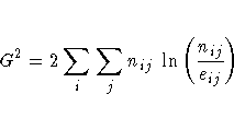
When the row and column variables are independent, G² has an asymptotic chi-square distribution with (R-1)(C-1) degrees of freedom. In addition to the asymptotic test, PROC FREQ computes the exact test when you specify the LRCHI or CHISQ option in the EXACT statement.

Continuity-Adjusted Chi-Square Test

The continuity-adjusted chi-square statistic for 2 ×2 tables is similar to the Pearson chi-square, except that it is adjusted for the continuity of the chi-square distribution. The continuity-adjusted chi-square is most useful for small sample sizes. The use of the continuity adjustment is controversial; this chi-square test is more conservative, and more like Fisher's exact test, when your sample size is small. As the sample size increases, the statistic becomes more and more like the Pearson chi-square.

The statistic is computed as

$Q_C = \sum_i \sum_j \frac { [ \max (0,| n_{ij} - e_{ij}|-0.5) ]^2} { e_{ij}}$

Under the null hypothesis of independence, Q_C has an asymptotic chi-square distribution with (R-1)(C-1) degrees of freedom.

Mantel-Haenszel Chi-Square Test

The Mantel-Haenszel chi-square statistic tests the alternative hypothesis that there is a linear association between the row variable and the column variable. Both variables must lie on an ordinal scale. The statistic is computed as

Q_MH = (n-1)r²

where r² is the Pearson correlation between the row variable and the column variable. For a description of the Pearson correlation, see the "Pearson Correlation Coefficient" section. The Pearson correlation and, thus, the Mantel-Haenszel chi-square statistic use the scores that you specify in the SCORES= option in the TABLES statement.

Under the null hypothesis of no association, Q_MH has an asymptotic chi-square distribution with 1 degree of freedom. In addition to the asymptotic test, PROC FREQ computes the exact test when you specify the MHCHI or CHISQ option in the EXACT statement.

Refer to Mantel and Haenszel (1959) and Landis, Heyman, and Koch (1978).

Fisher's Exact Test

2 × 2 Tables

For 2 ×2 tables, Fisher's exact test is the probability of observing a table that gives at least as much evidence of association as the one actually observed, given that the null hypothesis is true. The row and column margins are assumed to be fixed. The hypergeometric probability, p, of every possible table is computed, and the p-value is defined as

${PROB} = \sum_A p$

For a two-sided alternative hypothesis, A is the set of tables with p less than or equal to the probability of the observed table. A small two-sided p-value supports the alternative hypothesis of association between the row and column variables.

One-sided tests are defined in terms of the frequency of the cell in the first row and first column (the (1,1) cell). For a left-sided alternative hypothesis, A is the set of tables where the frequency in the (1,1) cell is less than or equal to that of the observed table. A small left-sided p-value supports the alternative hypothesis that the probability of an observation being in the first cell is less than expected under the null hypothesis of independent row and column variables.

Similarly, for a right-sided alternative hypothesis, A is the set of tables where the frequency in the (1,1) cell is greater than or equal to that of the observed table. A small right-sided p-value supports the alternative that the probability of an observation being in the first cell is greater than expected under the null hypothesis.

Because the (1,1) cell frequency completely determines the 2 ×2 table when the marginal row and column sums are fixed, these one-sided alternatives can be equivalently stated in terms of other cell probabilities or ratios of cell probabilities. The left-sided alternative is equivalent to an odds ratio greater than 1, where the odds ratio equals (n₁₁ n₂₂ / n₁₂ n₂₁). Additionally, the left-sided alternative is equivalent to the column 1 risk for row 1 being less than the column 1 risk for row 2, p_1|1 < p_1|2. Similarly, the right-sided alternative is equivalent to the column 1 risk for row 1 being greater than the column 1 risk for row 2, p_1|1 > p_1|2. Refer to Agresti (1996).

R × C Tables Fisher's exact test was extended to general R ×C tables by Freeman and Halton (1951), and this test is also known as the Freeman-Halton test. For R ×C tables, the two-sided p-value is defined the same as it is for 2 ×2 tables. A is the set of all tables with p less than or equal to the probability of the observed table. A small p-value supports the alternative hypothesis of association between the row and column variables. For R ×C tables, Fisher's exact test is inherently two-sided. The alternative hypothesis is defined only in terms of general, and not linear, association. Therefore, PROC FREQ does not compute right-sided or left-sided p-values for general R ×C tables.

For R ×C tables, PROC FREQ computes Fisher's exact test using the network algorithm of Mehta and Patel (1983), which provides a faster and more efficient solution than direct enumeration. See the section "Exact Statistics" for more details.

Phi Coefficient

The phi coefficient is a measure of association derived from the Pearson chi-square statistic. It has the range $-1 \leq \phi \leq 1$ for 2 ×2 tables. Otherwise, the range is $0 \leq \phi \leq min(\sqrt{R-1}, \sqrt{C-1})$ (Liebetrau 1983). The phi coefficient is computed as

$\phi = \frac{n_{11} n_{22} - n_{12} n_{21} } {\sqrt{n_{1 \cdot} n_{2 \cdot} n_{\cdot 1} n_{\cdot 2}}} {{\rm for 2 x 2\space tables}}$

$\phi = \sqrt{Q_P / n} {{\rm otherwise}}$

Refer to Fleiss (1981, pp. 59 -60).

Contingency Coefficient

The contingency coefficient is a measure of association derived from the Pearson chi-square. It has the range $0 \leq P \leq \sqrt{(m - 1)/m}$ , where m = min(R,C) (Liebetrau 1983). The contingency coefficient is computed as

$P = \sqrt{ \frac{Q_P}{Q_P + n} }$

Refer to Kendall and Stuart (1979, pp. 587 -588).

Cramer's V

Cramer's V is a measure of association derived from the Pearson chi-square. It is designed so that the attainable upper bound is always 1. It has the range $-1 \leq V \leq 1$ for 2 ×2 tables; otherwise, the range is $0 \leq V \leq 1$ . Cramer's V is computed as

$V = \phi {for 2 x 2\space tables}$

$V = \sqrt{ \frac{Q_P/n}{\min(R-1,C-1)} } {otherwise}$

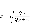
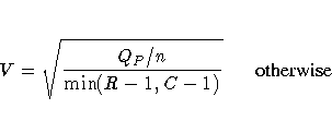
Refer to Kendall and Stuart (1979, p. 588).

Chapter Contents
Previous
Next
Top