Example 38.4: Automatic Smoothing Parameter Selection

The LOESS Procedure

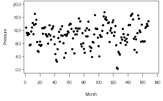
Example 38.4: Automatic Smoothing Parameter Selection

The following data set contains measurements of monthly averaged atmospheric pressure differences between Easter Island and Darwin, Australia for a period of 168 months (NIST 1998).

   data ENSO;
     input Pressure @@;
     Month=_N_; 
     format Pressure 4.1;
     format Month 3.0;
   datalines;
   12.9  11.3  10.6  11.2  10.9   7.5   7.7  11.7
   12.9  14.3  10.9  13.7  17.1  14.0  15.3   8.5 
    5.7   5.5   7.6   8.6   7.3   7.6  12.7  11.0
   12.7  12.9  13.0  10.9  10.4  10.2   8.0  10.9
   13.6  10.5   9.2  12.4  12.7  13.3  10.1   7.8
    4.8   3.0   2.5   6.3   9.7  11.6   8.6  12.4
   10.5  13.3  10.4   8.1   3.7  10.7   5.1  10.4
   10.9  11.7  11.4  13.7  14.1  14.0  12.5   6.3
    9.6  11.7   5.0  10.8  12.7  10.8  11.8  12.6
   15.7  12.6  14.8   7.8   7.1  11.2   8.1   6.4 
    5.2  12.0  10.2  12.7  10.2  14.7  12.2   7.1
    5.7   6.7   3.9   8.5   8.3  10.8  16.7  12.6
   12.5  12.5   9.8   7.2   4.1  10.6  10.1  10.1   
   11.9  13.6  16.3  17.6  15.5  16.0  15.2  11.2
   14.3  14.5   8.5  12.0  12.7  11.3  14.5  15.1
   10.4  11.5  13.4   7.5   0.6   0.3   5.5   5.0
    4.6   8.2   9.9   9.2  12.5  10.9   9.9   8.9
    7.6   9.5   8.4  10.7  13.6  13.7  13.7  16.5  
   16.8  17.1  15.4   9.5   6.1  10.1   9.3   5.3
   11.2  16.6  15.6  12.0  11.5   8.6  13.8   8.7 
    8.6   8.6   8.7  12.8  13.2  14.0  13.4  14.8
   ;

The following PROC GPLOT statements produce the simple scatter plot of these data, displayed in Output 38.4.1.

 
   symbol1 color=black value=dot ;  
   proc gplot data=ENSO;
      plot Pressure*Month /  
           hminor = 0
           vminor = 0
           vaxis  = axis1
           frame;
           axis1 label = ( r=0 a=90 ) order=(0 to 20  by 4);;
   run;

Output 38.4.1: Scatter Plot of ENSO Data

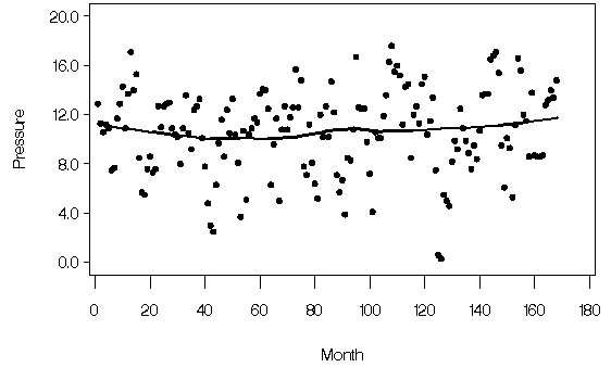
You can compute a loess fit and plot the results for these data using the following statements:

   ods output OutputStatistics=ENSOstats;

   proc loess data=ENSO;
      model Pressure=Month ;
   run;

   symbol1 color=black value=dot h=2.5 pct;  
   symbol2 color=black interpol=join value=none width=2;
   proc gplot data=ENSOstats;
      plot (depvar pred)*Month / overlay 
           hminor = 0
           vminor = 0
           vaxis  = axis1
           frame;
           axis1 label = ( r=0 a=90 ) order=(0 to 20  by 4);
   run; quit;

Output 38.4.2: Oversmoothed Loess Fit for the ENSO Data

You see that the default smoothing parameter 0.5 is too large. There are several strategies that you can use to select the smoothing parameter. The strategy used in the previous examples is to examine plots of the fit residuals versus the predictor variable and to choose the largest smoothing parameter that yields no clearly discernible trends in the fit residuals.

Alternatively, a variety of automatic methods for choosing the smoothing parameter exist. Many of these methods choose a smoothing parameter that minimizes a criterion that incorporates both the tightness of the fit and model complexity of the form

$\log( {\hat \sigma}^2 ) + \psi(L)$

where ${\hat \sigma}^2$ is the average residual sum of squares and $\psi(\cdot)$ is a penalty function designed to decrease with increasing smoothness of the fit. Here L is the smoothing matrix of the method. This matrix satisfies

$\hat{y}=L y$

where y is the vector of observed values and $\hat{y}$ is the corresponding vector of predicted values of the dependent variable. Examples of specific criteria obtained with this methodology are generalized cross validation (Craven and Wahba 1979), the Akaike information criterion (Akaike 1973), and the bias corrected Akaike information criteria (Hurvich and Simonoff 1998).

Hurvich and Simonoff (1998) show that the bias corrected Akaike information criteria avoid the tendency to undersmooth that often occurs when using the classical Akaike information criterion or generalized cross validation. One such criterion is given by

$AIC_{C_1} = n \log ( {\hat \sigma}^2 ) + n \frac {\delta_1/\delta_2(n+\nu_1)}{\delta_1^2/\delta_2-2}$

where

$n & \equiv & {Number of observations} \ \delta_1 & \equiv & {Trace} (I-L)^T(I-L)... ... \nu_1 & \equiv & {Equivalent number of parameters} \ & \equiv & {Trace} (L^T L)$

The statistics that you use to compute AIC_C₁ are also used to perform statistical inference in loess models. You can find these numbers in the "Fit Summary" table of PROC LOESS, provided that you specify at least one of the options ALL, CLM, DFMETHOD=EXACT, STD, and T in the MODEL statement. As with all tables of output, you can capture the "Fit Summary" table numbers in a SAS data set by using an ODS output. The following SAS macro takes such an output data set as an argument. It finds the smoothing parameter that yields the smallest AIC_C₁ statistic for all the smoothing parameters that you specify in the MODEL statement.

   %macro SmoothSelect(data); 
   options nonotes;
   ods listing close; 

   data temp;  
      set &data(keep = Label1 nValue1 smoothingParameter
         where=(Label1 in 
               ('Number of Observations',
                'Residual Sum of Squares',
                'Trace[L]'
                'Equivalent Number of Parameters',
                'Delta1',
                'Delta2',
                'Lookup Degrees of Freedom'))); 
   run;
    
   proc transpose data=temp(drop=Label1) out=temp;
      by smoothingParameter;
   run;

   data temp(drop=_NAME_); set temp;
      rename Col1 = n
             Col2 = rss
             Col3 = traceL
             Col4 = delta1
             Col5 = delta2
             Col6 = nu1
             Col7 = lkdf; 

   data SmoothCriteria(keep = SmoothingParameter aicc1);  
      set temp;
      sigmaHat=rss/n;
      aicc1=n*(log(sigmaHat) + (delta1/delta2)*(n+nu1)/(lkdf-2) );

   proc sort data=SmoothCriteria(where=(aicc1^=.))
                  out=Aicc1Results; 
      by aicc1;
   run;

   ods listing;
   proc print data=Aicc1Results(obs=1);
      title2 'Smoothing Parameter Minimizing the AICC1 Statistic'; 
      id SmoothingParameter;  
   run; 

   proc sort data=Aicc1Results; 
     by SmoothingParameter;
   run;

   title1 'AICC1 Criterion';
   symbol1 c=black i=join value=none width=2;
   proc gplot data=SmoothCriteria;
      plot aicc1*SmoothingParameter/
         hminor = 0
         vminor = 0
         vaxis  = axis1
         frame;
         axis1 label = ( r=0 a=90 );
   run; quit; 

   title1; 
   %mend;

You can use this macro as follows:

   proc loess data=ENSO;
      ods output fitsummary=ENSOsummary;
      model Pressure=Month /
          smooth = 0.03 to 0.1 by 0.01 
          dfmethod=exact;
   run;

   %SmoothSelect(EnsoSummary);

You use the DFMETHOD=EXACT option in the MODEL statement to produce the statistics needed to compute the AIC_C₁ criterion. You use the SMOOTH= option to specify the list of smoothing parameters you want to examine. You use the ODS OUTPUT statement to capture the "Fit Summary" tables for these smoothing parameters in the data set that you use as the argument for the SMOOTHSELECT macro.

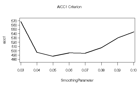
You obtain the plot shown in Output 38.4.3 and the output shown in Output 38.4.4.

Output 38.4.3: AIC_C₁ Statistic for the ENSO data

Output 38.4.4: Smoothing Parameter Minimizing the AIC_C₁ Statistic

Smoothing Parameter Minimizing the AICC1 Statistic

SmoothingParameter	aicc1
0.05	487.424

From Output 38.4.4 you see that 0.05 is the best smoothing parameter among the loess fits you requested. You can plot the loess fit for this smoothing parameter with the following statements:

   ods output OutputStatistics=ENSOstats;

   proc loess data=ENSO;
      model Pressure=Month/ smooth =0.05;
   run;

   symbol1 color=black value=dot h=2.5 pct;  
   symbol2 color=black interpol=join value=none width=2;
   proc gplot data=ENSOstats;
      plot (depvar pred)*Month / overlay 
           hminor = 0
           vminor = 0
           vaxis  = axis1
           frame;
           axis1 label = ( r=0 a=90 ) order=(0 to 20  by 4);
   run; quit;
   run;

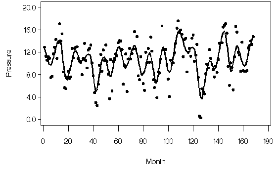
Output 38.4.5: Loess Fit with Smoothing Parameter 0.05

Chapter Contents
Previous
Next
Top