Multinormal Clusters of Unequal Size and Dispersion

Introduction to Clustering Procedures

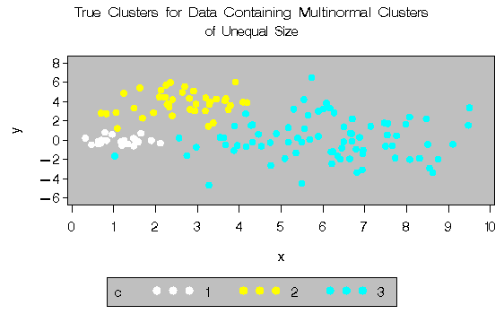
Multinormal Clusters of Unequal Size and Dispersion

In this example, there are three multinormal clusters that differ in size and dispersion. PROC FASTCLUS and five of the hierarchical methods available in PROC CLUSTER are used. To help you compare methods, the true, generated clusters are plotted. The following SAS statements produce Figure 8.9:

   data unequal;
      keep x y c;
      mx=1; my=0; n=20; scale=.5; c=1; link generate;
      mx=6; my=0; n=80; scale=2.; c=3; link generate;
      mx=3; my=4; n=40; scale=1.; c=2; link generate;
      stop;
   generate:
      do i=1 to n;
         x=rannor(1)*scale+mx;
         y=rannor(1)*scale+my;
         output;
      end;
      return;
   run;

   title 'True Clusters for Data Containing Multinormal 
          Clusters';
   title2 'of Unequal Size';
   proc gplot;
      plot y*x=c/frame cframe=ligr 
           vaxis=axis1 haxis=axis2 legend=legend1;
   run;

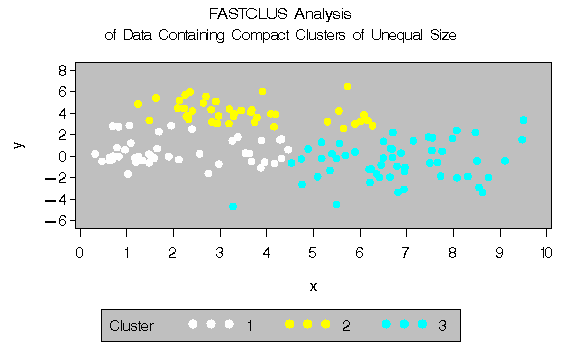
Figure 8.9: Data Containing Generated Clusters of Unequal Size

The following statements use the FASTCLUS procedure to find three clusters and the PLOTCLUS macro to plot the clusters. The statements produce Figure 8.10.

   proc fastclus data=unequal out=out maxc=3 noprint;
      var x y;
      title 'FASTCLUS Analysis';
      title2 'of Data Containing Compact Clusters of 
              Unequal Size';
   run;

   %plotclus;

Figure 8.10: Data Containing Compact Clusters of Unequal Size: PROC FASTCLUS

The following SAS statements produce Figure 8.11:

   proc cluster data=unequal outtree=tree 
                method=ward noprint;
      var x y;
   run;

   proc tree noprint out=out n=3;
      copy x y;
      title 'Ward''s Minimum Variance Cluster Analysis';
      title2 'of Data Containing Compact Clusters of 
              Unequal Size';
   run;

   %plotclus;

Figure 8.11: Data Containing Compact Clusters of Unequal Size: PROC CLUSTER with METHOD=WARD

The following SAS statements produce Figure 8.12:

   proc cluster data=unequal outtree=tree method=average 
                noprint;
      var x y;
   run;

   proc tree noprint out=out n=3 dock=5;
      copy x y;
      title 'Average Linkage Cluster Analysis';
      title2 'of Data Containing Compact Clusters of 
              Unequal Size';
   run;

   %plotclus;

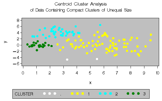
Figure 8.12: Data Containing Compact Clusters of Unequal Size: PROC CLUSTER with METHOD=AVERAGE

The following SAS statements produce Figure 8.13:

   proc cluster data=unequal outtree=tree 
                method=centroid noprint;
      var x y;
   run;

   proc tree noprint out=out n=3 dock=5;
      copy x y;
      title 'Centroid Cluster Analysis';
      title2 'of Data Containing Compact Clusters of 
              Unequal Size';
   run;

   %plotclus;

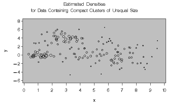
Figure 8.13: Data Containing Compact Clusters of Unequal Size: PROC CLUSTER with METHOD=CENTROID

The following SAS statements produce Figure 8.14:

   proc cluster data=unequal outtree=tree method=twostage 
                k=10 noprint;
      var x y;
   run;

   proc tree noprint out=out n=3;
      copy x y _dens_;
      title 'Two-Stage Density Linkage Cluster Analysis';
      title2 'of Data Containing Compact Clusters of 
              Unequal Size';
   run;

   %plotclus;

   proc gplot;
      bubble y*x=_dens_/frame cframe=ligr 
             vaxis=axis1 haxis=axis2 ; 
      title 'Estimated Densities';
      title2 'for Data Containing Compact Clusters of 
              Unequal Size';
   run;

Figure 8.14: Data Containing Compact Clusters of Unequal Size: PROC CLUSTER with METHOD=TWOSTAGE

The following SAS statements produce Figure 8.15:

   proc cluster data=unequal outtree=tree 
                method=single noprint;
      var x y;
   run;

   proc tree data=tree noprint out=out n=3 dock=5;
      copy x y;
      title 'Single Linkage Cluster Analysis';
      title2 'of Data Containing Compact Clusters of 
              Unequal Size';
   run;

   %plotclus;

Figure 8.15: Data Containing Compact Clusters of Unequal Size: PROC CLUSTER with METHOD=SINGLE

In the PROC FASTCLUS analysis, the smallest cluster, in the bottom left of the plot, has stolen members from the other two clusters, and the upper-left cluster has also acquired some observations that rightfully belong to the larger, lower-right cluster. With Ward's method, the upper-left cluster is separated correctly, but the lower-left cluster has taken a large bite out of the lower-right cluster. For both of these methods, the clustering errors are in accord with the biases of the methods to produce clusters of equal size. In the average linkage analysis, both the upper- and lower-left clusters have encroached on the lower-right cluster, thereby making the variances more nearly equal than in the true clusters. The centroid method, which lacks the size and dispersion biases of the previous methods, obtains an essentially correct partition.

Two-stage density linkage does almost as well even though the compact shapes of these clusters favor the traditional methods. Single linkage also produces excellent results.

Chapter Contents
Previous
Next
Top