Postscript version of this file

STAT 450 Lecture 3

Reading for Today's Lecture: Sections 1, 2 and 3 of Chapter 2. Sections 1 and 2 of Chapter 4.

Goals of Today's Lecture:

• Learn how to compute density of Y=g(X) from density of X when X and Y are real valued.

Last time: We defined:

• discrete distributions
• pmf: f(x) = P(X=x).
• absolutely continuous rv X
• density f: $P(X \in A) = \int_A f(x)\, dx$.

We introduced distribution theory

• X has known distribution
• Y=g(X) -- problem is to find distribution of Y.

Method 1: Two steps:

1.

Compute F_Y(y), the cdf of Y.

2.

Find f_Y(y) by differentiating F_Y.

For Y=g(X) with X and Y each real valued

$$P(Y \le y) = P(g(X) \le y) = P(X \in g^{-1}((-\infty,y]))$$

Take the derivative with respect to y to compute the density

$$f_Y(y) = \frac{d}{dy}\int_{\{x:g(x) \le y\}} f(x) \, dx$$

Often we can differentiate this integral without doing the integral.

Example: : 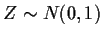$Z \sim N(0,1)$, i.e.

$$f_Z(z) = \frac{1}{\sqrt{2\pi}} e^{-z^2/2}$$

and Y=Z². Then

$$F_Y(y) = P(Z^2 \le y) = \left\{ \begin{array}{ll} 0 & y < ... ... P(-\sqrt{y} \le Z \le \sqrt{y}) & y \ge 0 \end{array}\right.$$

Now

$$P(-\sqrt{y} \le Z \le \sqrt{y}) = F_Z(\sqrt{y}) -F_Z(-\sqrt{y})$$

can be differentiated to obtain

$$f_Y(y) = \left\{ \begin{array}{ll} 0 & y < 0 \\ \frac{d}{dy... ...\right] & y > 0 \\ \mbox{undefined} & y=0 \end{array}\right.$$

Then

$$\begin{eqnarray*}\frac{d}{dy} F_Z(\sqrt{y}) & = & f_Z(\sqrt{y})\frac{d}{dy}\sqrt... ...frac{1}{2} y^{-1/2} \\ & = & \frac{1}{2\sqrt{2\pi y}} e^{-y/2} \end{eqnarray*}$$

with a similar formula for the other derivative. Thus

$$f_Y(y) = \left\{ \begin{array}{ll} \frac{1}{\sqrt{2\pi y}} e... ...0 \\ 0 & y < 0 \\ \mbox{undefined} & y=0 \end{array}\right.$$

We will find indicator notation useful:

$$1(y>0) = \left\{ \begin{array}{ll} 1 & y>0 \\ 0 & y \le 0 \end{array}\right.$$

which we use to write

$$f_Y(y) = \frac{1}{\sqrt{2\pi y}} e^{-y/2} 1(y>0)$$

(changing the definition unimportantly at y=0).

Notice: I never evaluated F_Y before differentiating it. In fact F_Y and F_Z are integrals I can't do but I can differentiate then anyway. You should remember the fundamental theorem of calculus:

$$\frac{d}{dx} \int_a^x f(y) \, dy = f(x)$$

at any x where f is continuous.

Method 2: Change of variables.

Now assume g is one to one. I will do the case where g is increasing and I will be assuming that g is differentiable. The density has the following interpretation (mathematically what follows is just the expression of the fact that the density is the derivative of the cdf):

$$f_Y(y) = \lim_{\delta y \to 0} \frac{P(y \le Y \le y+\delta y... ... \lim_{\delta y \to 0} \frac{F_Y(y+\delta y)-F_Y(y)}{\delta y}$$

and

$$f_X(x) = \lim_{\delta x \to 0} \frac{P(x \le X \le x+\delta x)}{\delta x}$$

Now assume that y=g(x). Then

$$P( y \le Y \le g(x+\delta x) ) = P( x \le X \le x+\delta x)$$

Each of these probabilities is the integral of a density. The first is the integral of the density of Y over the small interval from y=g(x) to $y=g(x+\delta x)$. Since the interval is narrow the function f_Y is nearly constant over this interval and we get

$$P( y \le Y \le g(x+\delta x) ) \approx f_Y(y)(g(x+\delta x) - g(x))$$

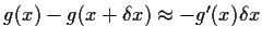
Since g has a derivative the difference

$$g(x+\delta x) - g(x) \approx \delta x g^\prime(x)$$

and we get

$$P( y \le Y \le g(x+\delta x) ) \approx f_Y(y) g^\prime(x) \delta x$$

On the other hand the same idea applied to the probability expressed in terms of X gives

$$P( x \le X \le x+\delta x) \approx f_X(x) \delta x$$

which gives

$$f_Y(y) g^\prime(x) \delta x \approx f_X(x) \delta x$$

or, cancelling the $\delta x$ in the limit

$$f_Y(y) g^\prime(x) = f_X(x)$$

If you remember y=g(x) then you get

$$f_X(x) = f_Y(g(x)) g^\prime(x)$$

or if you solve the equation y=g(x) to get x in terms of y, that is, x=g^-1(y) then you get the usual formula

$$f_Y(y) = f_X(g^{-1}(y)) / g^\prime(g^{-1}(y))$$

I find it easier to remember the first of these formulas. This is just the change of variables formula for doing integrals.

Remark: If g had been decreasing the derivative $g^\prime$ would have been negative but in the argument above the interval $(g(x), g(x+\delta x))$would have to have been written in the other order. This would have meant that our formula had $g(x) - g(x+\delta x) \approx -g^\prime(x) \delta x$. In both cases this amounts to the formula

$$f_X(x) = f_Y(g(x))\vert g^\prime(x)\vert \, .$$

The quantity $\vert g^\prime(x)\vert$ is called the Jacobian of the transformation g.

Example: $X\sim\mbox{Weibull(shape $\alpha$ , scale $\beta$ )}$or (see Chapter 3 for definitions of a number of ``standard'' distributions)

$$f_X(x)= \frac{\alpha}{\beta} \left(\frac{x}{\beta}\right)^{\alpha-1} \exp\left\{ -(x/\beta)^\alpha\right\} 1(x>0)$$

Let $Y=\log X$ so that $g(x) = \log(x)$. Setting $y=\log x$ and solving gives $x=\exp(y)$ so that g^-1(y) = e^y. Then $g^\prime(x) = 1/x$ and $1/g^\prime(g^{-1}(y)) = 1/(1/e^y) =e^y$. Hence

$$f_Y(y) = \frac{\alpha}{\beta} \left(\frac{e^y}{\beta}\right)^... ...a-1} \exp\left\{ -(e^y/\beta)^\alpha\right\} 1(e^y>0) e^y \, .$$

The indicator is always equal to 1 since e^y is always positive. Simplifying we get

$$f_Y(y) = \frac{\alpha}{\beta^\alpha} \exp\left\{\alpha y -e^{\alpha y}/\beta^\alpha\right\} \, .$$

If we define $\phi = \log\beta$ and $\theta = 1/\alpha$ then the density can be written as

$$f_Y(y) = \frac{1}{\theta} \exp\left\{\frac{y-\phi}{\theta} -\exp\left\{\frac{y-\phi}{\theta}\right\}\right\}$$

which is called an Extreme Value density with location parameter $\phi$ and scale parameter $\theta$. (Note: there are several distributions going under the name Extreme Value. If we had used $Y=-\log X$ we would have found

$$f_Y(y) = \frac{1}{\theta} \exp\left\{-\frac{y-\phi}{\theta} -\exp\left\{-\frac{y-\phi}{\theta}\right\}\right \}$$

which the book calls the Gumbel distribution.)

Marginalization

Now we turn to multivariate problems. The simplest version has $X=(X_1,\ldots,X_p)$ and Y=X₁ (or in general any X_j).

Theorem 1   If X has (joint) density $f(x_1,\ldots,x_p)$ then $Y=(X_1,\ldots,X_q)$ (with q < p) has a density f_Y given by

$$f_{X_1,\ldots,X_q}(x_1,\ldots,x_q) = \int_{-\infty}^\infty \c... ...-\infty}^\infty f(x_1,x_2,\ldots,x_p) \, dx_{q+1} \ldots dx_p$$

We call $f_{X_1,\ldots,X_q}$ the marginal density of $X_1,\ldots,X_q$ and use the expression joint density for f_X but $f_{X_1,\ldots,X_q}$ is exactly the usual density of $(X_1,\ldots,X_q)$. The adjective ``marginal'' is just there to distinguish the object from the joint density of X.

Example The function

f(x₁,x₂) = Kx₁x₂1(x₁> 0) 1(x₂ >0) 1(x₁+x₂ < 1)

is a density for a suitable choice of K, namely the value of Kmaking

$$P(X\in R^2) = \int_{-\infty}^\infty \int_{-\infty}^\infty f(x_1,x_2)\, dx_1\, dx_2 = 1 \, .$$

The integral is

$$\begin{eqnarray*}K \int_0^1 \int_0^{1-x_1} x_1 x_2 \, dx_1\, dx_2 & = & K \int_0... ...1(1-x_1)^2 \, dx_1 /2 \\ & = & K(1/2 -2/3+1/4)/2 \\ & = & K/24 \end{eqnarray*}$$

so that K=24. The marginal density of x₁ is

$$f_{X_1}(x_1) = \int_{-\infty}^\infty 24 x_1 x_2 1(x_1> 0) 1(x_2 >0) 1(x_1+x_2 < 1)\, dx_2$$

which is the same as

$$f_{X_1}(x_1) = 24 \int_0^{1-x_1} x_1 x_2 1(x_1> 0) 1(x_1 < 1) \, dx_2 = 12 x_1(1-x_1)^2 1(0 < x_1 < 1)$$

This is a $\mbox{Beta}(2,3)$ density.

The general multivariate problem has

$$Y=(Y_1,\ldots,Y_q) = ( g_1(X_1,\ldots,X_p), \ldots, g_q(X_1,\ldots,X_p))$$

Case 1: If q>p then Y will not have a density for ``smooth'' g. Y will have a singular or discrete distribution. This sort of problem is rarely of real interest. (However, variables of interest often have a singular distribution - this is almost always true of the set of residuals in a regression problem.)

Case 2 If q=p then we will be able to use a change of variables formula which generalizes the one derived above for the case p=q=1. (See below.)

Case 3: If q < p we will try a two step process. In the first step we pad out Y by adding on p-q more variables (carefully chosen) and calling them $Y_{q+1},\ldots,Y_p$. Formally we find functions $g_{q+1}, \ldots,g_p$ and define

$$Z=(Y_1,\ldots,Y_q,g_{q+1}(X_1,\ldots,X_p),\ldots,g_p(X_1,\ldots,X_p))$$

If we have chosen the functions carefully we will find that $g=(g_1,\ldots,g_p)$ satisfies the conditions for applying the change of variables formula from the previous case. Then we apply that case to compute f_Z. Finally we marginalize the density of Z to find that of Y:

$$f_Y(y_1,\ldots,y_q) = \int_{-\infty}^\infty \cdots \int_{-\in... ...f_Z(y_1,\ldots,y_q,z_{q+1},\ldots,z_p) \, dz_{q+1} \ldots dz_p$$