![]()
![]()
![]()
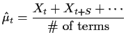
Model identification summary: The simplest model identification tactic is to look for either a pure MA or pure AR model. To do so:
If ![]() is not stationary we will need to transform
is not stationary we will need to transform ![]() to find a
related stationary series. We will consider in this course
two sorts of non-stationarity -- non constant mean and integration.
to find a
related stationary series. We will consider in this course
two sorts of non-stationarity -- non constant mean and integration.
Non constant mean: If
E![]() is not constant we
will hope to model
is not constant we
will hope to model
![]() E
E![]() using a small number of parameters
and then model
using a small number of parameters
and then model
![]() as a stationary series. Three common
structures for
as a stationary series. Three common
structures for ![]() are linear, polynomial and periodic:
are linear, polynomial and periodic:
Linear trend: Suppose
Method 1: regression (detrending). We regress
![]() on
on ![]() to get
to get
![]() and
and ![]() and analyze
and analyze
Method 2: differencing. Define

These random walk models are common in Economics. In physics they are used in the limit of very small time increments - this leads to Brownian motion.
Definition: ![]() satisfies an ARIMA
satisfies an ARIMA![]() model if
model if
Remark: If
![]() where
where ![]() is stationary
and
is stationary
and ![]() is a polynomial of degree
less than or equal to
is a polynomial of degree
less than or equal to ![]() then
then
![]() is stationary.
(So a cubic shaped trend could be removed by differencing 3 times.)
is stationary.
(So a cubic shaped trend could be removed by differencing 3 times.)
WARNING: it is a common mistake in students' data analyses to over
difference. When you difference a stationary ![]() you
introduce a unit root in the defining polynomial - the result
cannot be written as an infinite order moving average.
you
introduce a unit root in the defining polynomial - the result
cannot be written as an infinite order moving average.
Detrending: Define a response vector
![$\displaystyle U = \left[\begin{array}{c} X_0 \\ \vdots \\ X_{T-1} \end{array} \right]
$](img46.gif)
![$\displaystyle V=\left[\begin{array}{cc} 1 & 0 \\ 1 & 1 \\ \vdots & \vdots \\ 1 & T-1
\end{array}\right]
$](img47.gif)
![$\displaystyle Y = \left[\begin{array}{c} Y_0 \\ \cdots \\ Y_{T-1} \end{array} \right]
$](img49.gif)
![$\displaystyle \theta = \left[\begin{array}{c} \alpha \\ \beta\end{array}\right] \, .
$](img50.gif)
The problem in our context (it is almost always a problem)
is that you can only use
![]() if you know
if you know
![]() . In our context you won't know
. In our context you won't know ![]() until you
have removed a trend, selected a suitable
until you
have removed a trend, selected a suitable ![]() model and
estimated the parameters. The natural proposal is to follow
an iterative process:
model and
estimated the parameters. The natural proposal is to follow
an iterative process:
The process is repeated until the estimates stop changing in any important way.
Folklore: There is evidence that the OLS estimator has a variance which is not too much different from GLS in common ARMA models.
Every winter the measured (not reported) unemployment rate in Canada rises. A simple model which has this feature has a non-stationary mean of the form
Definition: Deseasonalization is the process of transforming ![]() to eliminate this sort of seasonal variation in the mean.
to eliminate this sort of seasonal variation in the mean.
Method 1: Regression. Estimate
![$\displaystyle \theta = \left[\begin{array}{c} \mu_0 \\ \vdots \\ \mu_{S-1}
\end{array}\right]
$](img70.gif)
![$\displaystyle V=\left[\begin{array}{ccccc} 1 & 0 & 0 & \cdots & 0
\\
0 & 1 & ...
...\
\vdots & \vdots & \vdots & \vdots & \vdots
\end{array}\right]_{T \times S}
$](img71.gif)
Method B: Seasonal differencing:
Definition: A multiplicative
![]() model has the form:
model has the form:
As an example consider the model
Fitting the ![]() part is easy we simply difference
part is easy we simply difference ![]() times. The
same observation applies to seasonal multiplicative model. Thus
to fit an ARIMA
times. The
same observation applies to seasonal multiplicative model. Thus
to fit an ARIMA![]() model to
model to ![]() you compute
you compute
![]() (shortening your data set by
(shortening your data set by ![]() observations)
and then you fit an
observations)
and then you fit an ![]() model to
model to ![]() . So we assume that
. So we assume that
![]() .
.
Simplest case: fitting the AR(1) model
Our basic strategy will be:
Generally the full likelihood is rather complicated; we will use conditional likelihoods and ad hoc estimates of some parameters to simplify the situation.
If the errors ![]() are normal then so is the series
are normal then so is the series ![]() . In general
the vector
. In general
the vector
![]() has a
has a
![]() where
where
![]() and
and ![]() is a vector all of whose entries are
is a vector all of whose entries are
![]() . The joint density of
. The joint density of ![]() is
is
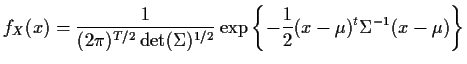
![$\displaystyle \ell(\mu,a_1,\ldots,a_p,b_1,\ldots,b_q,\sigma) =
-\frac{1}{2}\left[
(x-{\bf\mu})^t \Sigma^{-1} (x-{\bf\mu}) + \log(\det(\Sigma))\right]
$](img95.gif)
It is possible to carry out full maximum likelihood by maximizing the quantity in question numerically. In general this is hard, however.
Here I indicate some standard tactics. In your homework I will be asking you to carry through this analysis for one particular model.
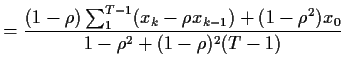
Consider the model
![$\displaystyle \ell(\mu,\rho,\sigma) = - \frac{1}{2\sigma^2}\sum_1^{T-1} \left[x_k-\mu-\rho(x_{k-1}-\mu)\right]^2
-(T-1)\log(\sigma) + \log(f_{X_0})
$](img102.gif)
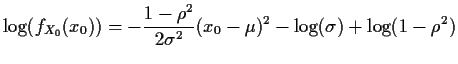
![$\displaystyle = - \frac{1}{2\sigma^2} \left\{ \sum_1^{T-1}\left[x_k-\mu-\rho(x_{k-1}-\mu)\right]^2 +(1-\rho^2)(x_0-\mu)^2\right\}$](img106.gif) |
||

+ (1-\rho^2)(x_0-\mu)\right\}
$](img109.gif)
 |
||
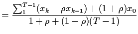 |
Now compute
![$\displaystyle \frac{\partial}{\partial\sigma} \ell = \frac{1}{\sigma^3}\left\{
...
...mu-\rho(x_{k-1}-\mu)\right]^2 +(1-\rho^2)(x_0-\mu)^2\right\}
-\frac{T}{\sigma}
$](img118.gif)
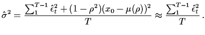
![$\displaystyle \hat\sigma^2(\rho) = \frac{\left\{
\sum_1^{T-1}\left[x_k-\mu(\rho)-\rho(x_{k-1}-\mu(\rho))\right]^2
+(1-\rho^2)(x_0-\mu(\rho))^2\right\}}{T}
$](img119.gif)
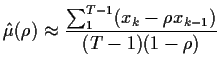
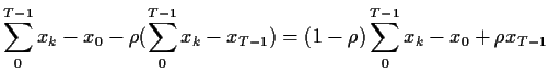
To find ![]() you now plug
you now plug
![]() and
and
![]() into
into ![]() (getting the so called profile likelihood
(getting the so called profile likelihood
![]() )
and maximize over
)
and maximize over ![]() . Having thus found
. Having thus found ![]() the mles of
the mles of ![]() and
and
![]() are simply
are simply
![]() and
and
![]() .
.
It is worth observing that fitted residuals can then be calculated: