The Cantor set (pp 67-72, 75-77). The Cantor set C can be constructed by removing the (open) middle third from [0,1] and then removing the middle thirds from the remaining intervals [0,1/3], [2/3,1], etc ad infinitum. The Cantor set is the set of points remaining. By adding up the lengths of the intervals removed (using the formula for a geometric series) we see that the "length" of C must be zero (because the lengths of all the intervals removed in the construction is 1).
Although the length of C is zero, there are many points in C. For instance, it's easy to see that the end points E = {0, 1, 1/3, 2/3, 1/9, 2/9, 7/9, 8/9, . . . } of the intervals removed are in C. But there are many, many more points in C (for example, 1/4 and 3/4 are in C). To find out exactly what points are in C, it is best to look at the ternary (or triadic) expansions of numbers in [0,1].
This way we see that the points in C have no 1 in their ternary expansion (since those regions of [0,1] containing numbers with a 1 in their ternary expansion were removed in the construction of C). Conversely, any number in [0,1] that has no 1 in its ternary expansion is in C. For those numbers that have two ternary expansions, if one of them has no 1 then that number is in C (for example, [1/3]3 = .1 or .022(22) ). It is important to note that any string .a1a2 a3. . . of 0's and 2's corresponds to (the ternary expansion of) a number in C.
Now we "match" the numbers in [0,1] to the numbers in C, in a one-to-one manner, to show that C contains at least as many points as [0,1]. To do that we first express numbers in [0,1] in base 2, i.e., we look at their binary expansions. So take any x in [0,1] and let [x]2 = .b1b2b3. . . be its binary expansion. Now we change every 1 that occurs in the binary expansion of x to a 2. Then we are left with a string .c1c2c3. . . of 0's and 2's (the c's that are 0 are in the same position as the 0's in the binary expansion of x). So this string must correspond to a (unique) number y in C where [y]3=.c1c2c3. . . .(because of the important note in the previous paragraph). Thus, we have matched every x in [0,1] to a (different) y in C and so the cardinality of [0,1] and C must be equal (i.e., the number of points in [0,1] and C must be the same).
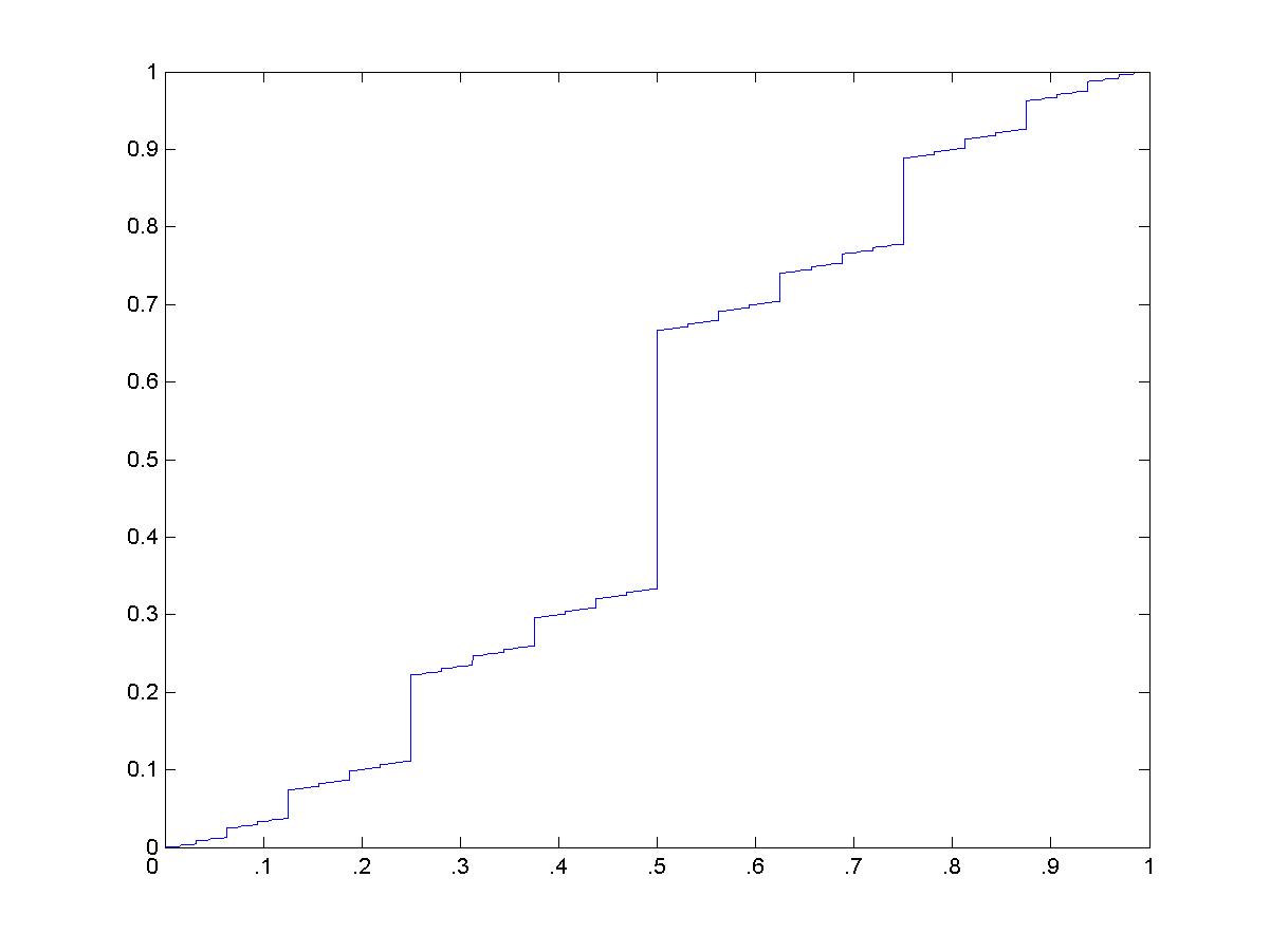
The graph of the function g: [0,1] to C via [x]2 goes to y in C by changing every '1' in [x]2 to a '2' to obtain [y]3; see page 75 in the text. Compare this to the 'Devil's Staircase', Figure 4.39 on page 226.(Click here for a larger view.) The MATLAB program that calculated this is here.
Properties of C;
- the length of C is zero
- C contains no intervals, i.e., is it "dust" ('totally disconnected' in mathematical jargon). Thus, between any two points in C is a point that is not in C.
- C has the same cardinality as [0,1]
- C is self-similar (i.e., small pieces of C are exact replicas - albeit on a smaller scale - of C)
- every point x in C is the limit of a sequence of end points. That is, there is an (infinite) sequence {yi} of points from E such that yi tends to x as i tends to infinity. So the end points "cluster" around the points in C.
Self-similarity (Chapter 3; pp 135-146). Here's a formal definition;
A set S in Rn is self-similar (or affinely self-similar) if there is a subset s of S, an (n by n) matrix A (or linear transformation) that is expanding, and a vector v in Rn, such thatThat is, a set is self-similar if a small piece of it is an exact replica of the entire whole (after expanding it and shifting it if necessary). This implies that the set is infinitely complicated; the small piece, being a replica of the whole, itself has a smaller piece which is a replica of the whole small piece, etc. We proved the self-similarity of the Cantor set using ternary expansions, and noted the self-similarity of the Sierpinski triangle and von Koch curve. Every fractal has this self-similarity (although sometimes it is not so obvious - for example, the fractal tree (also shown on page 242 of the text)). And, as we will see, many 'real' objects have some self-similarity.A(s) + v = S.(A linear transformation A is expanding if ||A(x)-A(y)|| is greater than ||x-y|| for all x,y in Rn.)
Some notes on using ternary expansions to prove the self-similarity of the Cantor set can be seen here; self_cantor.pdf, or self_cantor.jpg.
We started discussing the Sierpinski triangle (pp 78-79).
We discussed the von Koch curves (pp 89-93).
The Sierpinski triangle (pp 78,79) and the von Koch curve (pp 89-93, 147-152). Both were obtained by a recursive algorithm. The Sierpinski triangle contains an infinitely long curve (the edges of the triangles removed) and the von Koch curve is infinitely long. The von Koch curve intersects the interval [0,1] at exactly the Cantor set, and at each end point E of the intervals removed in the Cantor set construction (as described above) there is a corner of the von Koch curve. Keep in mind that the von Koch curve is a continuous curve and that the Cantor set is dust! So the von Koch curve is oscillating wildly (to put in mildly) along the interval [0,1]. That's what you need to do to fit an infinitely long curve into an area of finite size!
Measuring the complexity of curves (Section 4.2). Here we are after the exponent d in the relation log[u(s)] vs log(1/s). Here, u(s) is the length of the curve measured with rulers of size s (so if N(s) rulers of length s are needed to measure the length of the curve, u(s) = N(s)*s). We sometimes say that "u(s) is the length of the line at scale s". The exponent d is the slope of the (straight line part) of the curve that passes through the points when you plot log[u(s)] against log(1/s) (see Figures 4.12, 4.18 and 4.20 in the text). Note that if the data points (log[u(s)], log(1/s)) lie on a straight line of slope d, then log[u(s)] = d*log(1/s) + b, so (taking the exponential of both sides of this equation) u(s) = k*(1/s)d (here, k = eb). That is, u(s) is proportional to (1/s)d.
We saw that 'regular' curves have exponent d=0 and that 'fractal-like' curves have positive exponent; d>0. If d=0 then the length of the curve increases at the same rate at which the ruler used to measure the length shrinks (eg. if I shrink the size of the ruler by 3 (so it becomes 1/3 its previous length), the number of rulers needed to measure the length of the curve goes up by a factor of 3 too, etc). However, if d>0 then the number of rulers needed to measure the length of the curve increases at a faster rate than the rate at which the scale s is shrinking (for example, with the von Koch curve, if you shrink the scale by a factor of 3, the number of rulers you need goes up by a factor of 4). You can see this from the formula u(s) = c(1/s)d - so if you shrink the ruler from size s to size s/m, then the length of the line at this smaller scale is u(s/m) = c(1/(s/m))d = mdc(1/s)d = mdu(s); the length increases by a factor of md (here we are thinking of m >1).
See also last year's commentary; 14 January and 21 January.
Fractal Dimension (or self-similarity dimension) (Section 4.3). Here we are measuring the complexity of sets by covering them with small squares or cubes and counting how many of these small squares or cubes are needed to cover the set. We then shrink the size of these small squares or cubes and count again how many of these smaller squares and cubes are needed to cover the set. Of course, since the squares or cubes are shrinking in size we will need more of them to cover the set, but for some sets the increase in the number of small squares or cubes is greater than for other sets. The rate of increase in the number of small squares or cubes need to cover the set as they shrink in size is a measure of the complexity of the set; as our scale decreases in size we see the same or even more detail in complicated sets than for less complicated sets (i.e., 'regular' sets).
As for the length of curves, we expect a power law relation between the number of small squares or cubes needed to cover the set, a(s), and the size (or scale) if the small squares or cubes, s. That is, we expect a formula of the type u(s) = c(1/s)D for some D > = 0 (D will be greater or equal to zero since the number of small squares or cubes needed to cover the set increases as the scale shrinks). The exponent D is called the fractal dimension of the set.
To compute the fractal dimension of a set, you choose an (appropriate) sequence of scales sn such that sn -> 0 as n -> infinity, and count the minimum number of squares or cubes a(sn) that are needed to cover the set. Then you write a(sn) as a power law; u(sn) = c(1/sn)D for some constant c . The exponent D you find is the fractal dimension of the set. Note that we would just write u(s) = c(1/s)D; that is, just s instead of sn.
It's easy to calculate the fractal dimension of simple sets. For a line segment of length L we choose the scales sn = L/n, n=1, 2, 3, ... and cover it with line segments or squares or cubes of size sn. Here, a(sn) = n. We can write n = L/n = L(1/sn)1 so that a(s) = L(1/s)1 and so we see that the fractal dimension for a line is 1. For a square of size L we choose the same scales sn = L/n and cover the square with small squares or cubes of size sn. Here, a(sn) = n2 = L2(1/sn)2 so the fractal dimension of a square is 2. For a cube we find that a(sn) = n3 = L3 (1/sn)3 so the fractal dimension of a cube is 3. With a bit of help from calculus, we would find that the fractal dimension of any regular curve is 1, the fractal dimensio of any regular area is 2, and that the fractal dimension of any regular volume is 3. Thus, for regular sets the fractal dimension agrees with the topological dimension.
However, the topological dimension doesn't say anything about the complexity of a set, and that's what we are trying to study here (and what scientists in general are studying when they study fractals and chaos). For example, the von Koch curve, the Sierpinski triangle, and Peano's space filling curve (see pp 94) are all curves (i.e., they have topological dimension 1), but they are not anything like 'regular' curves because they are infinitely complicated; when you zoom in on them they look the same. Their complexity is reflected in their fractal dimensions; D = 1.26, 1.58, and 2 for the von Koch, Sierpinski and Peano curves respectively - von Koch is the least complicated of the three (but still infinitely more complicated than a regular curve), Sierpinski is the next most complicated, and the Peano curve is the most complicated of the three. In fact, the Peano 'curve' is more like an area than a line.
To get a better idea of what the fractal dimension is telling us about a set, let's consider the unit square [0,1]2 and the grids of size sn = (1/2)n that cover the square (the top part of Figure 4.30, pp 213, shows two grids; see also the examples given below). If A is any subset of [0,1]2, then to calculate the fractal dimension of A we cover it with grids of various sizes and count how many of the small squares of each grid (the minimum number) are needed to cover A. Then we calculate the exponent D as described above. But let's go backwards and start with the covering rather than with the set (let's remark that a covering at scale sn is just a selection of small squares from the grid of size sn). A consistent covering is a selection of covers from each grid size in such a way that in the covering at any scale only the small squares that are within the squares choosen for the covering at the previous step can be used. If you think about it, for any choice of consistent covering there is a set A that has that covering.
Doing this allows us, for one thing, to find a set A with prescribed fractal dimension. For example, if we wanted to find a set with fractal dimension (log 3)/(log 2) = 1.58, we would just choose a covering that had a(sn) = 3n squares at scale sn (because a(sn) = 3n = (1/sn) D = (2n)D for D = (log 3)/(log 2).) An important observation is that the fractal dimension only depends on the number a(sn) of squares choosen at each scale and not on their arrangement. This implies that you can find many sets with the same fractal dimension; just choose the a(sn) squares differently (but consistently!) when making a new covering. You can also get an idea of what the set A looks like that has that fractal dimension by sketching the coverings at smaller and smaller scales.
As an example, for each scale sn choose the 2n diagonal squares in the grid. This is a consistent covering and you can see that the set A = diagonal line has this covering. Since a(sn) = 2n = (1/sn)1, A has fractal dimension 1 (which we knew already). But we can rearrange the 2n squares at each scale in a consistent way to obtain the covering of another set B that also has fractal dimension 1. In fact, you can choose the covering so that B is not a line at all but in fact is dust!
Here are two examples of consistent coverings:
one with fractal dimension 1; JPEG format, PDF format,
and one with fractal dimension 1.5;
JPEG format, and PDF format . See here for a larger picture of the fractal set covered by the latter covering.
Another thing we can do here is try to get some idea of how much you can vary a covering without changing the fractal dimension. For example, suppose a1(sn) is the number of grid squares used at scale sn for a covering that gives fractal dimension D1. Suppose at each scale sn we remove k of the squares of that covering. Then we can conclude that no matter how large k is the fractal dimension of the resulting covering is still D1 (note that you could not begin removing the k squares until you reached a small enough scale m so that a1(sm) > k). We prove this in the case when the covering is for the entire square [0,1]2, so a1(sn) = 4n:
-
We start removing squares from the the original covering at some stage m where
k < a1(sm) = 4m.
Let a(s) denote the number of squares used at scale s in our new covering.
Then
-
a(sm) = 4m - k (so there are 4(4m - k) = 4m+1 - 4k
squares of size sm+1),
a(sm+1) = 4m+1 - 4k - k (so there are 4(4m+1 - 4k -k) squares of size sm+2),
...
...
...
a(sm+p) = 4n - k(4p + 4p-1 + . . . + 4 + 1) = 4n - k(4p+1-1/3), (n = m+p).
In practice, the fractal dimension of a set is often measured by the box counting method. See the Jan 21 commentary, W00 for discussion of this, and Section 4.4 of the text.
In practice, the fractal dimension of a set is often estimated by the box counting method (Section 4.4, pp 212-216; see also the 21 Jan 2000 commentary).
We started on Iterated Function Systems (IFS). To motivate this we considered the Multiple Reduction Copy Machine (MRCM) paradigm (see Sections 1.2 and 5.1 and the 28 Jan, 2000 commentary). This is a kind of photocopier that has several lenses, each one reduces the size of the object it images, and then the resulting images are arranged in some particular way on the resulting output. For example, the Sierpinski MCRM has three lenses, each one reduces to 1/2 size, and the resulting three images are arranged at the vertices of an equilateral triangle (see Figure 1.9). If you you feed the resulting image back into the MCRM over and over again, the output begins to look like the Sierpinski triangle (see Figures 1.10 and 5.1). In fact, all fractals can be obtained this way.
What characterizes an MCRM (and an IFS) is its blueprint (see page 238). The blueprint is simply the image of the unit square by the MCRM. For the Sierpinski MCRM the blueprint consistes of three squares of size 1/2 arranged in an equilateral triangle (see Figure 5.9, for example). If we indicate the orientation of the square by placing an 'L' in the top left corner, then the blueprint tells us everything about the MCRM (and IFS); how many lenses are involved, what each lens does (eg., shrink, rotation, reflection, etc.), and how the images produced by each lens are arranged in the output. It's important to note that the fractal produced by an MCRM (or IFS) is unchanged when imaged by that MCRM. This is really the only way to determine what kind of image is produced by an MCRM or IFS (we will discuss this more later).
Each lens of an MRCM is modelled mathematically by an affine transformation w which is a transformation of the form w = A + v where A is a (2 by 2) matrix and v is a vector (in R2). For most purposes, the matrices A can be realized as a composition of 'elementary' transformations like rotations, reflections, dilations (in both x and y directions), and shears (see page 234-236). The mathematical model of the MCRM is, then, an IFS W; W = w1 U w2 U . . . U wk where each wi=Ai+vi is an affine transformation (the matrices Ai and vectors vi may differ for each lens).
See Ch 5 and Section 3.4; and 28 January W00 commentary, and 2 Feb W01 commentary.
See here for examples of iterates of various IFS.
We looked at the problem of encoding an image as an IFS (Chapter 5). Here we are guided by the facts (which will be explained later) that if F is the image that is eventually drawn by the IFS W, then W(F) = F. Now, W is made up of several affine transformations wi of the form wi = A + v where A is a matrix and v is a vector (the shift); W = w1 U w2 U . . . wk (here, U denotes union - see page 238). So W(F) = F means that F = F1 U F2 U . . . U Fk where Fi = wi(F). Since each Fi is a smaller copy of F (and perhaps rotated, reflected, or sheared or a combination of these), we see that F is the union of smaller (perhaps distorted) copies Fi of itself: the IFS builds in the self-similarity of F. This allows us to find an IFS that draws F: break up F into k self-similar pieces Fi. Then figure out what the affine transformation wi are such that wi(F) = Fi. We use the parameters a,b,c,d,e,f to define an affine transformation w = A + v, where a,b,c,d are the entries of the matrix A (a=A11, b=A12, c=A21, d=A22), and e,f are the components of the vector v; v = (e,f). See page 295 in the text for a listing of the paramenters for the various IFS that draw the fractals in that chapter. See also Section 3.4 and the 28 January commentary for W00.
See here for examples of iterates of various IFS.
I did some experiments/examples of IFS's using the applets and VB programs available on the course webpage. Using the VB program Fractal Pattern, we saw the iteration of the IFS's that produce the Sierpinski triangle, the von Koch and square von Koch curves, and the Fern. We also looked at the IFS for the Cantor set and the Cantor line set (Cantor set stretched into lines). The parameters for these two IFS's are (since they are not in the menu);
- Cantor set:
- 1: (a, b, c, d, e, f, p) = (0.334, 0, 0, 0.334, 0, 0.334, 0.5)
- 2: (a, b, c, d, e, f, p) = (0.334, 0, 0, 0.334, 0.667, 0.334, 0.5)
- Cantor lines:
- 1: (a, b, c, d, e, f, p) = (0.334, 0, 0, 1, 0, 0, 0.5)
- 2: (a, b, c, d, e, f, p) = (0.334, 0, 0, 1, 0.667, 0, 0.5)
I did some experiments with the Fractal Movie applet. In the Fractal Movie applet you specify an initial (start pattern) IFS (or blueprint) and final (end pattern) IFS. The applet then interpolates between the two, drawing the fractal produced by the intermediatary IFS's. For the first experiment I simply took as initial IFS the Sierpinski IFS with top lens (#3) sitting all the way to the left and final IFS the Sierpinski IFS with lens #3 all the way to the right. The parameters were (only parameters for lens #3 need to be adjusted from the Sierpinski IFS parameters obtained from the drop down menu);
- start 3: (a, b, c, d, e, f, p) = (0.5, 0, 0, 0.5, 0, 0.5, 0.334)
- end 3: (a, b, c, d, e, f, p) = (0.5, 0, 0, 0.5, 0.5, 0.5, 0.334)
- start 3: (a, b, c, d, e, f, p) = (0.5, 0, 0, 0.5, 0, 0.5, 0.334)
- end 3: (a, b, c, d, e, f, p) = (0, -0.5, 0.5, 0, 0.5, 0.5, 0.334)
- 1: (a, b, c, d, e, f, p) = (0.85, -0.31, 0.31, 0.85, 0.2, -0.1, 0.5)
- 2: (a, b, c, d, e, f, p) = (0.35, -0.2, 0.2, 0.35, 0.5, 0.4, 0.5)
- end 2: (a, b, c, d, e, f, p) = (0.35, -0.2, 0.2, 0.35, -0.2, 0.4, 0.5)
- end 2: (a, b, c, d, e, f, p) = (0.35, -0.2, 0.2, 0.35, 0.5, 0, 0.5)
- end 2: (a, b, c, d, e, f, p) = (-0.2, -0.35, 0.35, -0.2, 0.7, 0.6, 0.5)
The Contraction Mapping Principle (see Section 5.6 and Jan 28 2000 commentary): If f is a contraction on the space X, then there exists a unique fixed point p of f, f(p) = p, and if x is any point in X then f n(x) -> p as n -> infinity. If A is an (n by n) matrix such that ||Ax-Ay||< ||x-y|| for any vectors x and y, then A is a contraction (on Rn). Since 0 is always a fixed point of any matrix, Anx -> 0 for any vector x for such an A. An affine transformation w = A + v is a contraction if and only if A is a contraction. Hutchinson's Theorem (p 268): If the wi are contractions on R2, then the IFS W = w1 U w2 U . . . U wk is a contraction on the space X of images (i.e., bounded subsets of R2) where distance between images is measured by the Hausdorff distance (p 268). And so this is why an IFS that is made up of contractions wi converges to an image F under iteration no matter what image you start with. Note that the image F is the fixed point of the IFS.
To find the fixed point of an affine transformation w = A + v, solve the equation w(p) = p; p = A(p) + v for p. To find the fixed point of an IFS W, iterate W beginning with any image S. However, as we will see, it may take the IFS a very long time to converge to the fixed point - so in the next chapter we will consider another method to ind the fixed point (final image) of an IFS. This is the problem of decoding an IFS (see page 259-260).
We defined the Hausdorff distance h(A, B) between two sets A and B: see pages 268 - 269. If e1 is the infimum of the set of e' s such that B is contained in the set Ae, and e2 is the infimum of the set of e' s such that A is contained in Be, then h(A,B)= max {e1, e2} (see page 269). Here, the infimum of a set (that is bounded from below) is the "bottom edge" of that set. Note that the infimum of a set may not be in that set, for example, the infimum of the set (1,2) is 1 (see also page 216). For example, the Husdorff distance between two points A={p} and B={q} is the distance between the two points; h(A,B)=||p-q||. If a set B is contained in a set A, then the set of all e' s such that B is contained in Ae is (0, infinity), so the infimum of this set, e1, is 0. Now, suppose we remove a single point from the set A, call this new set C, so that B is no longer contained in C (one point of B is not covered by C). Then still e1 = 0 because still the set of all e' s such that B is contained in Ce is (0, infinity). In the example done in class today, A was a (solid) square with sides of length 2r and B was the (solid) disc of radius r enscribed within the square, the centre of the square and the centre of the disc coinciding. Then h(A,B) = sqrt(2)r - r = e2 (note that e1=0). Now, if C is the square minus the center point, then (still) e2 = sqrt(2)r-r and e1=0, so h(C,B)=sqrt(2)r-r. So we see that the Hausdorff distance does not distinguish between sets that are "too close" together - for example, adding or removing finitely many points from one of the sets may not change the Hausdorff distance between the sets (more about the consequence of this next time).
We discussed the Collage Game (Section 5.8). This is the problem of making an IFS that generates a certain image. To begin with, we break-up the image into self-similar pieces and look for (affine) transformations wi that produce these images. In practice, the transformations wi are determinend interactively, i.e., by testing them to see what kind of image the IFS produces (see Fig 5.47) and then changing the parameters (a, b, c, d, e, f) to obtain a better image. In addition to obtaining fractals this way (in fact, the result will also be a fractal), one can obtain images that look very much like `realistic' objects (see Fig 5.49 where an image of a leaf is reproduced by an IFS with 7 lenses).
Decoding an IFS is the problem of drawing the image produced by an IFS (see pages259-260 and 4 Feb W2000 commentary). Recall that by Hutchinson's Theorem, if the wi are all contractions on R2 with respect to the Euclidean metric (or norm, or distance; these are all synonyms for metric), then the IFS W = w1 U w2 U . . . U wk is a contraction on the space X of images in R2 with respect to the Hausdorff metric, and so iterating the IFS will ultimately lead to the fixed point F of the IFS. However, the rate at which the iterates Wn(S) converge to the image F delends on how much W contracts (with respect to the Hausdorff metric). This could be so slow that it could take literally forever to draw the fractal F this way. We can easily compute how many iterations are required to draw the fractal F by first calculating how many iterations are required for the initial image S (say, the unit square) to be the size of one pixel (on your computer screen), and then calculating how many images (squares, if S is a square) will be drawn after this many iterations of the IFS. For Sierpinski, if S is a square 5002, then because the contractions of the wi are 1/2, you need about 9 iterations before the initial square S is of size 1 (so, (1/2)9*500 <= 1). So the total number of squares drawn is 1 + 3 + 32 + . . . + 39 = (310-1)/(3-1) which is about 30,000. Assuming the computer can draw 10,000 squares per second, the compter needs about 3 seconds to draw the Sierpinski triangle. However, since the slowest contraction in the Ferm IFS is only .85, you need about 39 iteations before the intial square S is 1 pixel small. The number of squares drawn will 1 + 4 + 42 + . . . + 4 39 which is about 1023. To draw this many squares with your computer would require more time than the age of the universe...... We will see in the next chapter that another method to draw fractals, the Chaos Game, always works.
Fractal Image Compression. Compression means storing data on a computer using the least amount of memory possible. Images contain a lot of data (8 bits per pixel for grey-scale image, so a 512x512 pixel ('bitmap') image contains about 260KB (kilobytes; 1 byte is 8 bits) of data) so finding an efficient way to store them on a computer (and so being able to electronically transmit them efficiently) is important. The JPEG image compression standard can compress images by a factor of between 5 and 15 (depending on the image) without perceptible distortion (so a 260KB bitmap image can be stored as JPEG file of size around 18KB to 52KB). Fractal image compression takes advantage of the approximate self-similarity present in most (natural) images. If an image was exactly self-similar, then you only need the IFS that has that image as a fixed point to 'store' the image (everytime you want to see the image you just run the IFS). An IFS is just a collection of numbers that define the transformations wi, and they don't take up much memory. For example, the bitmap of the Sierpinski triangle requires several hundred KB of data, the JPEG image would require several 10's of KB of data, but the IFS requires only 3 x 6 = 18 numbers! (this is about 100 bytes) Very roughly, the idea of fractal image compression is to partition the image into non-overlapping 'ranges' Ri (say, of size 4x4 pixels square) and then compare every 8x8 pixel square 'domain' Dj of the image to each range Ri. Affine transformations wi are applied to each domain Dj to try to match the Ri to Dj. Once a satisfactory domain and transformation is found for that range Ri, you move on to the next range Ri+1. When you are done with all the ranges you create a (big!) IFS W = w1 U w2 U. . . U wk. When iterated (begining with any initial image S) you will obtain an image that approximates the original image. See the references for examples and more description. The best fractal image compression schemes have compression ratios comparable to the best JPEG schemes today.
References: See S. Mallat's book A Wavelet Tour of Signal Processing, Second Ed. Section11.4 for more (technical) information about image compression. For fractal image compression see Appendix A of the text (PJS), the books, Fractal Image Compression by Yuval Fisher, or Fractal and Wavelet Image Compression Techniques by Stephen Welstead, SPIE Optical Engineering Press, 1999, the U of Waterloo website http://links.uwaterloo.ca, and the reports by Andrew Dagleish and Farhad Sadaghaini .
See some examples of fractal image compression on the Fractal Image Compression page.
We began the next chapter, Chapter 6: The Chaos Game. We have seen that iterating an IFS may not be the best way to draw a fractal (in fact, the Fern fractal can not be drawn this way). The problem there is that some wi of the IFS may contract too slowly. A 'chaos game' is an initial point z0, an IFS W = w1 U w2 U . . . U wk, a set of probabilities p1, p2, . . . pk (so 0 < pi < 1 and p1 + p2 + . . . + pk = 1), and a 'random' sequence {s1, s2, . . . , sn} of numbers from the set {1, 2, ..., k} (i.e, each si is choosen randomly from {1, 2, ..., k} according to the probabilities p1, ..., pk). The sequence of points {z0, z1, . . . , zn}, where zi = wsi(zi-1), is the outcome of the chaos game. We saw that several thousand points zi are needed to see the fractal clearly (so n is usually several tens of thousands - or even hundreds of thousands). The applets on the software webpage use the chaos game to draw fractals. (See the 21 Feb W2000 commentary for discussion of the chaos game.)
Some examples of using The Chaos Game method to draw fractals.
To understand why the chaos game 'works' (i.e., why it draws the fractal), we need to introduce the notion of addresses on a fractal. If W = w1 U w2 U . . . U wk is the IFS of the fractal F, then the region wt1(wt2( ... wtm(F))...) (which we may sometimes write as wt1wt2...wtm(F) - this is the composition of the w's acting on F) of F has address t1t2... tm. Note that you read an address from left to right to locate the region with that address on the fractal, but the transformations are applied from right to left. See pages 310-314 in the text.
Now note that if z is any point in the fractal F, then wt1(wt2( ... wtm(z))...) is a point in the region of the fractal that has address t1t2... tm (because z is inside of F and the simple fact that if p is a point in a set A, then w(p) is a point in the set w(A)). Thus, if we begin the chaos game with a point z0 in F, and if the random sequence {s1, s2, . . . , sn} is used in the game (i.e., these si are the random numbers choosen), then z1 is in the region of F with address s1 (because z1 = ws1(z0)), z2 is in the region of F with address s2s1 (because z2 = ws2(z1) = ws2(ws1(z0))), z3 is in the region of F with address s3s2s1 etc., and zn is in the region of F with address snsn-1, . . . s2s1. So the random sequence {s1, s2, . . . , sn} tells us the addresses of the game points {z1, z2, . . . , zn} (but note that all we know about the address of z1 is that it begins with s1, all we know about the address of z2 is that it begins with s2s1, all we know about the address of z3 is that it begins with s3s2s1, etc; if we want more precise addresses of the game points than this we need to know the address of the initial point z0).
A consequence of this is that if a certain string tmtm-1. . . t2t1 appears in the sequence {s1, s2, . . . , sn}, then we know that some game point will land in the region of F with address t1t2. . . tm-1 tm.
Now we can explain why the game points {z1, z2, . . . , zn} eventually (i.e., as n tends to infinity) "fill" the fractal F. We will do the proof for the Sierpinski Chaos game. To do this we pick any point p in T (the Sierpinski triangle) and any small number d. We want to show that some game point lies within a distance d of p. First pick m such that (1/2)m < d. Because each wi of the Sierpinski IFS contracts by 1/2, any region on T with address of length k will be of size (1/2)k, so any region of T with address of length m will be smaller than d. Let t1t2. . . tm-1tm be the first m digits in the address of p. Thus, p lies in the small triangle with address t1t2. . . tm-1tm. Now, as explained above, if the string tmtm-1. . . t2t1 appears in the sequence {s1, s2, . . . }, then some game point will land in this small triangle with address t1t2. . . tm-1tm. Thus, this game point will be within d of the point p (because this small triangle has size (1/2)m). But why should the string tmtm-1. . . t2t1 appear in {s1, s2, . . . }? It appears because of the following fact about random sequences:
-
If p1, p2, . . . pk are the probabilities that the digits
1, 2, . . . , k are chosen randomly for the sequence {s1, s2, . . . },
then the string tmtm-1. . . t2t1 will appear in the sequence with
frequency ptmpt(m-1)...pt2pt1 (this is the product of the
probabilities ptm, pt(m-1), . . . , pt1.)
In short, a game point will land in every address region of the fractal because every string that can be made from the digits {1,2,...,k} will appear (infinitely many times in fact!) in the sequence {s1, s2, s3, . . . }.
See also page 317 in the text.
Some examples of using The Chaos Game method to draw fractals.
Recall that to play a Chaos Game, you need an IFS W = w1 U w2 U . . . U wk, a set of probabilities p1, p2, . . . , pk, an initial game point z0, and a sequence of random numbers {s1, s2, . . . , sn} where the si are chosen according to the probabilities p1, p2, . . . , pk. Then one obtains the game points {z1, s2, . . . , zn} according to the rule zk+1 = ws_(k+1)(zk). All that was needed to prove that the game points will eventually fill-out the fractal F (F is the fixed point of the IFS: W(F) = F) is that every possible finite string of the digits 1, 2, ..., k appear in the sequence {s1, s2, . . . } (we proved this using addresses of the fractal F: the region Ft1...tm of F with address t1t2... tm is the set Ft1...tm = wt1wt2...wtm(F)).
See the handouts page for some (more) notes on the chaos game. (Note: The HW problems listed there are not to be handed in.)
The probability that a certain string, say tmtm-1...t1, appears in the sequence {s1, s2, . . . }, is the product of probabilities ptm pt(m-1)...t1. So for example, if p1=.2, p2=.3 and p3= .4, then the probability that the string 213 appears in {s1, s2, . . . } is p2p1p3 = (.3)(.2)(.4) = .024 (so this string will occur, on average, 2.4% of the time, or about 24 times in every sequence of length 1000). Note that this means that 2.4% of the game points will fall in the region with address 312.
So we can estimate the number of game points needed to fill-out the fractal on our computer screen. Suppose we are playing the chaos game with the Sierpinski IFS and the fractal fills the screen 512 by 512 pixels. Each wi contracts by 1/2, so regions on F with addresses of length k will be of size (1/2)k*(512). When this product is 1, the regions are of size one pixel so we can not discerne regions with addresses of longer lengths. In this example, address of length 9 will be 1 pixel in size. So we only need from our random sequence all strings of length 9 made from the digits 1, 2, 3. Then we will draw the Sierpinski as accurate as our computer screeen allows. So how long must the random sequence {s1, s2, . . ., sn} be so that it contains all strings of length 9? Well, the probability that the string t9t8...t2t1 appears is pt9pt8...pt2pt1. Since all the probabilities pi are equal to 1/3 (in this case), the probability that any string of length 9 will appear in the random sequence {s1, s2, . . ., sn} is (1/3)9 or about 1/20,000. So the length, n, should be around 20,000 (we will need about 20,000 game points to draw the Sierpinski triangle). See pages 316-317 in the text.
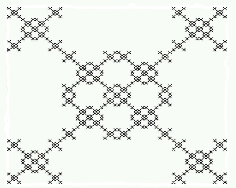
We considered the "full triangle" IFS on the Modified Chaos Game applet. Here there are 4 lenses. The first 3 lenses are the same as in the Sierpinski IFS, and the fourth lens fills the triangle in the centre. When we play this chaos game we will generate a random sequence {s1, s2, . . ., sn} of digits from {1,2,3,4}. Since the solid triangle is a fixed point of this IFS (check!), the game points of the chaos game with this IFS will eventually fill-out the solid triangle (try it). Now, if we remove all the 4's from the sequence {s1, s2, . . ., sn} we will be left with a (random) sequence of digits from {1,2,3}. This sequence with the full triangle IFS will produce the Sierpinski triangle (since you will be doing the same thing as you would with the Sierpinski chaos game). Removing all 4's from the sequence {s1, s2, . . ., sn} means that no strings containg a 4 will occur, which in turn means that no game point will land in a region of the full triangle with address containing a 4. If you think about it, removing all regions with addresses that contains a 4 will leave you with exactly the Sierpinski triangle (so the Sierpinski triangle is the full triangle minus all the regions with addresses that contain a 4). Now instead of removing all 4's from the sequence {s1, s2, . . ., sn}, what happens if we remove all occurences of the string '12'? Then no string that conntains a 12 will occur, which means no game point will land in a region of the full triangle with address containing a 21 in it. For example, you will see 'holes' in the full triangle that correspond to regions with address 21, 211, 213, 121, 1121, 2111, etc. See the Modified Chaos Game applet and the figure there. If you look closely you will see that this is NOT a fractal. But it has some kind of self-similarity.
We discussed how to express the game rules of a chaos game in plain English. That is, starting with an IFS, can you write-down the game rules in plain English? To do this, we first expressed the affine transformations wi = Ai + (ei, fi) in terms of just Ai and the fixed point qi. Since wi(qi) = qi, Ai(qi) + (ei, fi) = qi, so that (ei, fi) = qi - Ai(qi). So wi = Ai + qi - Ai(qi) - this is the affine transformation expressed in terms of just Ai and qi. So the mathematical chaos game rule zk+1 = wi(zk) can be written as zk+1 = qi + Ai(zk-qi), which in English says, "standing on qi, go to Ai(zk-qi) to obtain zk+1" (you have to express the formula Ai(zk-qi) in English).
The next topic is adjusting the probabilities in the chaos game (Section 6.3). Suppose we play the chaos game with the Sierpinski IFS, but instead of using equal probabilities p1 = p2 = p3 = 1/3 (like we have been), we use the probabilities p1 = p2 = 0.2, p3 = 0.6. Then 3 will occur in the random sequence {s1, s2, . . . } 3 times as often as a 1 or a 2 will occur. Consequently, game points will land in the region with address 3 (the top part of the triangle) 3 times as often as they will land in the regions with address 1 or 2. So playing the chaos game with these probabilities will result in the top part of the Sierpinsli triangle filling out more quickly than the bottom parts (try this with the applet, or look at Figure 6.21 on page 324 of the text, and the Chaos Game with Varying Probabilities page given below). The proof that the chaos game draws the fractal only used the property that the probabilities are non-zero, so the Sierpinski triangle WILL be drawn - but it will take a lot longer to draw than if equal probabilities were used. We can go on. The string 13 will occur 3 times as often in {s1, s2, . . . } as the string 12, so 3 times as many game points will land in the region with address 31 than in the region with address 21. The string 133 will occure 9 times as often in {s1, s2, . . . } as the string 122, so 9 times as many game points will land in the the region with address 331 than in the region with address 221, etc. These kind of calculations explain the image you see when you run the applet with these probabilities.
See the Chaos Game with Varying Probabilities page for some examples of fractals drawn with the chaos game using unusual probabilites.
I ran the chaos game using the full square IFS (i.e., an IFS with 4 lenses whose blueprint fills the initial square). The fixed point of this IFS is clearly the full square. Since all contractions are equal, the best probabilities used to draw this fractal are the equal ones; pi = 1/4. We know that the chaos game with any (non-zero) probabilities will (eventually) draw the full square, but you get vastly different intermediate patterns if you choose non-equal probabilities. For example, choose instead p1=p2=.4 and p3=p4=.1 (here, lens 1 is in the bottom left corner, lens 2 is in the top left corner, lens 3 is in the top right corner, and lens 4 is in the bottom right corner - just as they are on the Chaos Game and Fractal Movie applets), you will see a whole series of vertical lines. We can understand this pattern by realizing that most of the time, the sequence is just 1's and 2's (in fact 80% of the time) so points will move towards the fixed point (the line) of the IFS made of just lens 1 and 2. But whenever a 3 or 4 comes along in the sequence, the game point (which is lying very near that vertical line on the left edge) will jump towards one of the corners on the right edge of the square (these are the fixed points of the lenses 3 and 4). They will move 1/2 the distance towards them, in fact (lenses are contractions by 1/2). Thus, they will lie along the vertical line at x = 1/2. The vertical line at x=3/4 is caused by game points on the line x=1/2 under one of the transformations 3 or 4 (which move them again 1/2 the distance towards the fixed points). That's why you see a whole series of vertical lines at x=1/2, x=3/4, x=7/8, x=15/16, .... Homework problem #11 in Homework #3 is similar to this.
We discussed playing the chaos game with the Sierpinski IFS using the sequence s = {1,2,3,1,2,3,1,2,3,.....} (that is, 123 repeating). Suppose the initial game point z0 is somewhere inside the full triangle T0. Then the addresses of the game points {z1, z2, z3, ....} are 1_ _ , 21_, 321, 1321, 21321, 321321, 1321321, .... . We see that the game points are approaching the three points p1, p2, p3 with addresses 32132132...., 213213213....., and 132132132..... (because the addresses of the game points are agreeing more and more with the addresses of these three points as the game proceeds). Now, playing the chaos game with the sequence s = {1,2,3,1,2,3....} is like applying the transformation w321 = w3w2w1 over and over again beginning with the initial game point z0, or like applying the transformation w213 = w2w1w3 beginning with the second game point z1, or like applying the transformation w132 = w1w3w2 to the third game point z2. So those three points are the fixed points of these three (contractive, affine) transformations; w321(p1)=p1, w213(p2)=p2, w132(p3)=p3 (note that applying anyone of these three transformations shifts the address of a point to the right by three places, so check that the addresses of these fixed points is unchanged when the transformation is applied to it).
Adjusting probabilities (see Section 6.3 in the text). For IFS whose transformations have all the same rate of contraction, we saw that when the probabilities are all equal the fractal is drawn most efficiently (over other, non-equal probabilities). However, if the transformations have differing rates of contractions, then we gave heuristic arguments to show that, at least in some approximation, that choosing the probabilities pi such that the ratios p1/c1, p2/c2, ... , pk/ck are all equal, and that p1 + p2 + . . . pk = 1 (so that the pi's are probabilities) gave a good impression of the fractal (here we are considereing regions of address length 1). Here ci = |det Ai|, the absolute value of the determinent of the matrix Ai of the transformation wi, is the factor by which wi changes areas. The argument was to make the densities of points in the parts of the fractal with addresses of equal length the same.
- (Density is number of points/ area of region; if N is the number of game points
used in the game, then the number of points in the region with address i is pi*N, and
if a is the area of the filled in fractal FF,
then the area of the region with address i is area of(wi(FF)) = ci*area of(FF)
= ci*a (see Figure 5.38 on page 280 of the text),
so density = (pi*N)/(ci*a); when we equate these together, we can cancel out the
common factors N and a; that's why we only need to consider the ratios
pi/ci.)
In class we calculated the probabilities which gives equal densities of game points for all regions of the fern with address length 1. However, even though the adjusted probabilities insure that the density of game points in each region of address length 1 have equal densities, the densities of points within those regions (i.e., regions of address lengths greater than 1) may have non-equal densities. If you want to insure, in addition, that regions of address length 2 have equal densities, then you will have to solve the equations (p1p2/c1c2) = (p1p3/c1c3) = . . . . We also have to require that p1 + p2 + . . . pk = 1. See pages 327-329, and Section 6.5 of the text for a discussion of the 'Adaptive Cut' method for drawing the fractal very efficiently with the chaos game.
Playing the chaos game with sequences that are not random.
See the Chaos Game with Non Random Sequences handout.
Recall that the only property needed of the sequence {si} in order that the fractal gets drawn when using this sequence in the chaos game, was that it contain every possible string of the integers {1,..., k} (where the IFS has k transformations). Actually, if your computer screen can only resolve detail down to level 'm' (i.e., addresses of length m are the smallest areas you can see; they are about one pixel in size), then you only need a sequence that contains all possible strings of length m (then a point will land in each of these addresses when the chaos game is played with that sequence). One can write down a sequence that contains all strings of length m; the 'naive' sequence will be of length kmm . However, there will be a lot of redundancy from using such a string in the chaos game (for example, suppose we want to draw Sierpinski triangle to level 3, then the naive sequence has 33 3 = 81 numbers, from which we will obtain 81 points. However, there are only 27 addresses of length 3, so we only need 27 points). There are 'best' sequences that have no redundancies. Such sequences have length km + m-2. Note this is about km for moderately large m, which is smaller by a factor of m than the length of the 'naive' sequences.
How well do random sequences do? As explained in the handout (and as you will see if you do Problem # 16 on Homework #3), they do an intermediate job. That is, to draw a fractal to a certain degree of completeness, the length of a random sequence needed to do this will be longer than the 'efficient' (or 'best') one but shorter than the 'naive' one.
Some references about these topics;
- A Probabilist Looks at the Chaos Game, by Gerald Goodman, in the book, Fractals in the Fundamental and Applied Sciences, edited by H.-O. Peitgen, J.M. Henriques, and L.F. Penedo.
- Rendering Methods for Iterated Function Systems, by D. Hepting, P. Prusinkiewicz, and D. Saupe in the same book as above.
End of Fractal section of course.
Summary for Dynamics