Spatial Analysis__________________________________________________________________________
Three Multi-Criteria Evaluations were carried out, the first weighting more heavily on forested areas, wetlands, parks, and water. The second analysis used a more moderate weighting scheme. The third analysis weighted more heavily on agriculture and urban areas. The analytical hierarchy process (AHP) was used to determine the weighting scheme, as well as ordered weighted averaging (OWA). The AHP method uses a pairwise comparison approach to determine the weights of the various factors. The continous rating scale ranges from 1/9 being extremely less important, to 1 which is equally important, to 9 being extremely important, while the OWA weights applies weights on a pixel by pixel basis to the order of suitability scores (order weight 1 would be the lowest). The OWA weights used are provided in the table below:
weight 1 |
weight 2 |
weight 3 |
weight 4 |
weight 5 |
weight 6 |
weight 7 |
weight 8 |
weight 9 |
0.0080 |
0.0080 |
0.0150 |
0.0700 |
0.0920 |
0.0970 |
0.1700 |
0.2400 |
0.3000 |
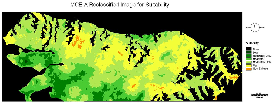
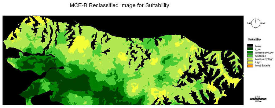
Once the suitability image was produced, it was then reclassed into an image that is more easily understood for which areas are the most suitable. The same reclass values were used for each image so they could be compared to each other with more ease. The new values range from unsuitable to most suitable.
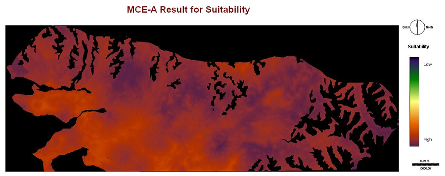
MCE-A Suitability Analysis: Heavily Weighted on Forested Areas, Wetlands, Parks, and Water
Below is the table of pairwise comparisons for analysis A, and its resulting eigenvector of weights.
agriculture_fuzz |
main _parks_fuzz |
old_fuzz |
young_fuzz |
urban_fuzz |
wet_fuzz |
roads_fuzz |
water_fuzz |
lesser_parks_fuzz |
|
agriculture_fuzz |
1 |
||||||||
main_parks_fuzz |
6 |
1 |
|||||||
old_fuzz |
7 |
2 |
1 |
||||||
young_fuzz |
6 |
1 |
1/3 |
1 |
|||||
urban_fuzz |
1 |
1/6 |
1/7 |
1/5 |
1 |
||||
wet_fuzz |
8 |
3 |
2 |
3 |
8 |
1 |
|||
roads_fuzz |
2 |
1/5 |
1/6 |
1/4 |
2 |
1/6 |
1 |
||
water_fuzz |
9 |
5 |
3 |
5 |
9 |
3 |
7 |
1 |
|
lesser_parks_fuzz |
5 |
1/3 |
1/3 |
1/2 |
5 |
1/3 |
4 |
1/5 |
1 |
The eigenvector of weights is :
agriculture_fuzz: 0.0189
main_parks_fuzz: 0.1010
old_fuzz: 0.1528
young_fuzz: 0.0865
urban_fuzz: 0.0192
wetlands_fuzz: 0.1936
roads_fuzz: 0.0281
water_fuzz: 0.3339
lesser_parks_fuzz: 0.0659
Consistency ratio = 0.05
Consistency is acceptable.
The resulting suitability is shown below.
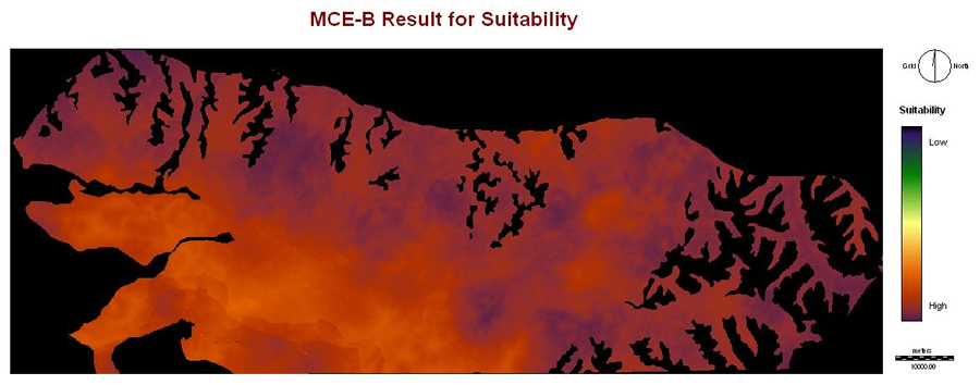
MCE- B Suitability Analysis: Moderate Weighting
Below is the table of pairwise comparisons for analysis A, and its resulting eigenvector of weights.
agriculture_fuzz |
main _parks_fuzz |
old_fuzz |
young_fuzz |
urban_fuzz |
wet_fuzz |
roads_fuzz |
water_fuzz |
lesser_parks_fuzz |
|
agriculture_fuzz |
1 |
||||||||
main_parks_fuzz |
1/5 |
1 |
|||||||
old_fuzz |
3 |
2 |
1 |
||||||
young_fuzz |
1/4 |
1 |
1/3 |
1 |
|||||
urban_fuzz |
1 |
4 |
1/3 |
3 |
1 |
||||
wet_fuzz |
3 |
2 |
1 |
3 |
1 |
1 |
|||
roads_fuzz |
1/6 |
1/3 |
1/5 |
1/4 |
1/5 |
1/5 |
1 |
||
water_fuzz |
3 |
5 |
3 |
4 |
3 |
2 |
6 |
1 |
|
lesser_parks_fuzz |
1/5 |
1/3 |
1/5 |
1/2 |
1/5 |
1/3 |
3 |
1/6 |
1 |
The eigenvector of weights is :
agriculture_fuzz: 0.1255
main_parks_fuzz: 0.0555
old_fuzz: 0.1733
young_fuzz: 0.0520
urban_fuzz: 0.1222
wet_fuzz: 0.1462
roads_fuzz: 0.0224
water_fuzz: 0.2700
lesser_parks_fuzz: 0.0330
Consistency ratio = 0.07
Consistency is acceptable.
The resulting suitability is shown below.
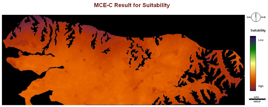
MCE-C Suitability Analysis: Heavily Weighted on Agricultural and Urban Areas
Below is the table of pairwise comparisons for analysis A, and its resulting eigenvector of weights.
agriculture_fuzz |
main _parks_fuzz |
old_fuzz |
young_fuzz |
urban_fuzz |
wet_fuzz |
roads_fuzz |
water_fuzz |
lesser_parks_fuzz |
|
agriculture_fuzz |
1 |
||||||||
main_parks_fuzz |
1/4 |
1 |
|||||||
old_fuzz |
1/3 |
2 |
1 |
||||||
young_fuzz |
1/5 |
1 |
1/3 |
1 |
|||||
urban_fuzz |
1 |
5 |
4 |
3 |
1 |
||||
wet_fuzz |
1/4 |
2 |
1 |
3 |
1/4 |
1 |
|||
roads_fuzz |
1/3 |
2 |
2 |
1/2 |
1/3 |
2 |
1 |
||
water_fuzz |
1 |
3 |
2 |
3 |
1 |
1 |
2 |
1 |
|
lesser_parks_fuzz |
1/5 |
1/3 |
1/4 |
1 |
1/3 |
1/2 |
1/2 |
1/2 |
1 |
The eigenvector of weights is :
agri_fuzz: 0.2216
main_parksfuzz: 0.0528
old_fuzz: 0.0885
young_fuzz: 0.0567
urban_fuzz: 0.2157
wet_fuzz: 0.0854
roads_fuzz: 0.0895
water_fuzz : 0.1472
lesser_parks_fuzz: 0.0426
Consistency ratio = 0.07
Consistency is acceptable.
The resulting suitability is shown below.
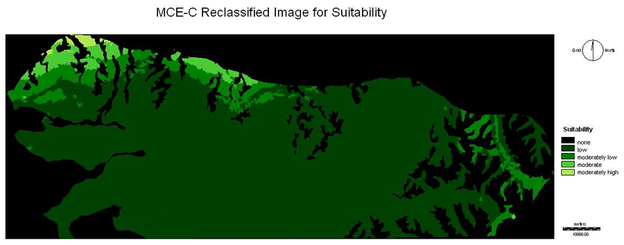
The results all show a higher suitability to the north and east of the Fraser River Valley, most likely because these areas have had the least, if not any, development. Analysis A presents the greatest amount of suitable areas, while analysis C presents the least amount of suitable areas. Analysis A could be representative of someone in agriculture or land development because they would want to show that there are still suitable habitat locations where the Pacific Water Shrew can live. Analysis C could be representative of a conservationist, showing that there are not many suitable habitat locations and that action should be taken against further land development.
Jacquelyn Shrimer ~ jshrimer@sfu.ca ~ Geog 355