In
the
previous module, we began investigating some of the many ways
in which time delays are involved in both acoustic and
electroacoustic processes, and that rather surprisingly result
in a wide range of perceptual effects, ranging from timbral
alterations in the very short domain (via phasing), spatial
effects with reflections in the medium range, rhythmic
effects with echo in a longer range, and by extension,
larger patterns over time, as summarized in the pdf introduced in the
previous module.
In the acoustic module on Sound-Environment Interaction, we
provided a summary of the acoustic processes in enclosed and
semi-enclosed spaces that produce the sound field
known as reverberation.
Multiple reflections, all of which are frequency dependent,
based on the nature of the space, its walls, floor and
ceiling, along with all objects within the space, combine to
spread throughout the space and reinforce the sound produced
within it. In a sense, reverberation is the complex aural
image created by the space itself. If you are not
familiar with how this process works, check out sections B and C in that module.
The main psychoacoustic effect of reverberation is to increase
the perceived magnitude or volume
of sounds in a space. It does so by prolonging the sound,
thereby adding loudness, and spectral colouration, as well as
blending multiple sounds together. In the electroacoustic
world, dry synthesized sounds are often in need of such
enhancement.
However, in the acoustic tradition, all soundmaking within the
space must adapt itself optimally to the reverberant
conditions, in terms of speed, dynamic range and timbral
articulation. In other words, soundmaking, particularly with
speech, cannot be independent of the acoustic space.
Too much reverberation can reduce speech comprehension and
muddy a musical ensemble. In subjective tests, listener
preferences are aimed at combining a sense of envelopment
in the right balance with definition and intimacy.
Too much of one reduces the other.
In the electroacoustic world, there are no such constraints,
so it is up to the sound designer’s sensibility to create the
optimal balance. We will cover the topic and its applied
aspects in these sub-topics.
A) Reverberation in the
analog and digital domains
B) Impulse Reverberation
C) Studio demo's of reverberation
D) Studio demo's of impulse reverb
Q) Review quiz
home
A. Reverberation: Analog and Digital. As
described in the last module, time delays, such as those
involved with sound reflections, require some form of memory.
In the early 20th century, such storage was difficult to
implement, not only for audio but also early computing
research. In the early broadcasting industry, as described by
Emily Thompson in The Soundscape of Modernity, radio
stations preferred to avoid using reverberation with
their monophonic signals, and hence fitted out their studios
with absorbent material to provide a dry acoustic. Given the
problem of static and low bandwidth for the radio signal,
reverberation was deemed to be a detriment for the listener –
essentially a form of noise.
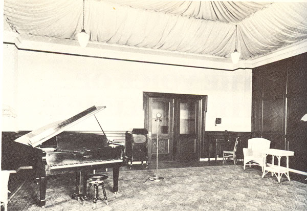
The CNRV radio recording studio, Vancouver, ca. 1925 with a
ceiling that is acoustically treated.
Another solution that was developed in the 1940s and 50s was
the spring reverberator and the plate
reverberator, both of which used an electromechanical
transducer to transfer the signal into a metal spring or
plate at one end, and retrieve it via a contact microphone
or pickup at the other end. The spring reverb unit, being
smaller, was pioneered for the Hammond Organ.
Large plate reverberators, such as those produced by EMT in
Germany, were more sophisticated and included a damping
mechanism connected to the very large metal sheets. Smaller
units were often included in electroacoustic music studios
as well, but it was the use of specific units in pop music
in the 1950s and 60s that established the mystique attached
to the specific sound of these units. Of course, their
frequency response was far from neutral, and with the
smaller units, reverb time couldn’t be controlled. These
specialized forms of reverb are often imitated in today’s
reverb plug-ins.
Digital audio and digital
reverberation started developing in the 1970s, and its
techniques are beyond our scope in terms of details. One of
the main pioneers, Barry Blesser, has devoted a chapter in
his book, co-authored with Linda-Ruth Salter, Spaces
Speak: Are You Listening, to the historical
development of high-end digital reverberation and makes for
interesting reading. Today, numerous reverb plug-ins
are available, each with their own set of variables, ranging
from simplistic to bewilderingly detailed. It is also
typical that presets are offered for specific types
of spaces or specific vocal or instrumental sources, such
that reverb is often simply chosen from a menu, not
specifically designed.
As with many issues in the electroacoustic world,
justification and intention is often expressed in the
language of fidelity,
such as “realism”, while at the same time the
operational reality is to enhance and essentially
create an artificial realism. With sufficient exposure, such
artificiality becomes normalized and familiar, and simply
part of cultural experience. In a previous module, this was
referred to as a “normalization of the artificial”.
The purpose here is not to say whether this is good or bad,
but simply to compare audio practice with everyday aural
experience.
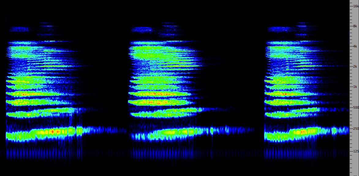
Here’s an interesting place to start: three examples of a
mezzo-soprano voice with added reverberation. In the next
section, we will discuss impulse reverberation as an
example of convolution,
also a form of digital processing. For each of the three
examples, try to determine if it is artificially produced by
a digital algorithm, or if it is modelling an actual space
via convolution. In each case, we've chosen a large church
acoustic with a long reverb.
A
B
C
(Source:
Sue
McGowan)
|
Click
to enlarge
|
First of all, it’s clear you have to listen
carefully to hear the differences. Examples A and C are
algorithmically produced, A with the ubiquitous DVerb
plug-in using these settings,
and C with the AirRvb plug-in using these settings. In each
case the direct signal was lowered by 12 dB to simulate the
distance from the mike involved in the convolved version (B)
whose Impulse Response was recorded in an Italian cathedral,
as seen here. Note that
the AirRvb reverb time was lowered to 5 seconds, because at
8 seconds, it simply lasted too long.
Two main differences to notice are that a high-frequency
boost was added to the SoundHack convolved example (B), but
slightly rolled off to be less bright. The algorithmic
versions, however, seem to emphasize the “bite” of the
initial attack such that the voice seems closer than
the convolved version which actually does sound at the
distance of the microphone from the source as predicted.
In each algorithmic case, there was zero pre-delay
added. This is the term used to delay the onset of the
reverb to avoid masking, but it also seems to serve in this
case to maintain the close presence of the voice, rather
than move it back in space.
So, did you have a preference? The algorithmic versions
clearly have a super smooth form of reverb, but the question
remains as to whether you want this effect on everything you
use it for. I think it’s clear that the impulse reverb with
convolution has the advantage of sounding very different for
each space that has about the same reverb time.
The frequency response of each acoustic space is highly
different, but in most plug-ins, there is a limited array of
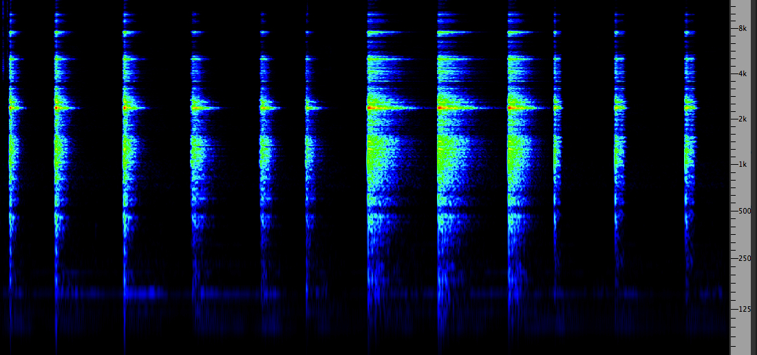
spectrum controls. In the simplest cases, we get a generic
choice, for instance in the following example of (1) bright
(emphasized highs); (2) dark (de-emphasized highs);
(3) large warm (emphasized mid-range with longer
reverb time); (4) gated.
Four
reverb
types: bright, dark, warm, gated
|
Click
to enlarge
|
The gated
case is, of course, entirely artificial as it cannot happen
in the acoustic world. That is, the reverb is added only
during the duration of the original sound, and removed
(i.e. gated out) immediately following. This enriches the
timbre of the original with no possibility of the reverb
masking or muddying the following sounds.
Digital reverberation algorithms today
can easily produce the kind of echo density of
reflections that are required – ideally more than 1000/sec.
A density that is too low produces a fluttering
effect. The early digital delay lines discussed in the last
module, such as the Lexicon, could only use feedback and
modulation of its two delay lines, so the quality of
reverberation was quite limited.
As discussed in the Sound-Environment Interaction module, good
concert hall acoustics include early reflections
arriving within the first 100 ms. Late arriving reflections
should have smooth decay with high frequency energy falling
off faster than the lows. A typical circuit proposed as
early as the 1960s by Manfred Schroeder included comb
filters in parallel (to simulate early reflections), and
cascaded all-pass filters to synthesize reverb. However,
many other models, including those involving feedback have
been proposed.

In small and medium sized rooms,
resonances known as eigentones are predominant
because of the smaller dimensions, as discussed here. In larger rooms,
reverberation is dominant. However, some tunnels exhibit
both characteristics because of their length. Here is a
final example of how resonance and reverberation can
interact, recorded by in the vaults of the National Library
in Vienna.
Tunnel inside the National Library, Vienna (Source
WSP Eur 23-24)
|
Click
to enlarge
|
Index
B. Impulse Reverberation. Impulse
reverb, also known as Convolution Reverb, is a
technique that involves convolving an acoustically dry sound
with the impulse response (IR) of a space. Normally
the IR is a recording of a short, broadband sound with a
strong attack, such as breaking a balloon, but it can also
be derived from a theoretical calculation of the properties
of an acoustic space based on its size and component
materials.
An acoustician could use a starter pistol as a source, but
for obvious reasons that is not practical or advisable for
an individual. Informally, a handclap is commonly used to
test out the acoustics of a space because it is short
enough, and broadband enough, to hear the frequency response
of the space and its reverberation time. However, for more
precise testing, a standardized and repeatable sound is
needed.
Reverberation time is how long it takes the sound to
die away, that is, to decay to -60 dB of its original
strength, but what is more important in the IR is the
frequency colouration the space provides, as this can be
quite complex.
You can hear a set of IR examples here in the Sound-Environment Module,
if you haven’t done so already. Then return and listen to
this set of examples of
vocal sounds processed with them and others.
Convolution then is a mathematical model of exactly what
happens to sound in an acoustic space, hence the realism of
the results. It follows the principle that the spectra of
the sound and the IR are multiplied together, and
that the resulting duration is the sum of the
durations of the sound and the IR, as you would expect from
reverberation lengthening a sound. Multiplying the spectra
is what we mean when we say that some frequencies are
emphasized and some attenuated in an acoustically bright or
dark room.
The apparent distance of the
source sound that results from the convolution is the same
as the distance the original source (e.g. balloon) was from
the microphone that recorded it. For sound production, this
can seem like a limitation, as we are used to moving sounds
around in a virtual space. The options for doing this with
impulse reverb (as the process is usually called) are:
-
technically you need an IR recording for several positions
and distances in the space; some IR catalogues provide
this, but it is not common
- in
the vocal sound examples in the previous webpage, there
were two that showed that if you convolve a sound with the
same IR twice, it will appear to be at double the
distance, so that technique could be used with
cross-fading
- the
most common way of moving a sound closer or farther from
the listener is to adjust the so-called dry/wet mix,
that is, the relative proportions of the original sound
and the reverberated portion. The reverberated part is
usually kept constant and the dry component varied; the
stronger the dry sound is, the closer the sound will
seem. For very large distances, the reverb signal
should also be slowly attenuated. Most impulse reverb apps
will provide this, because it is easy and effective. In
fact the psychoacoustic cue for distance, even in a
monophonic dimension, is so strong and we are so used to
it, that moving a sound towards or away from the listener
is easily achieved
- in a
DAW mix, you can multitrack both versions, dry and
wet, that is, original and reverberated, and then adjust
the level of the original in any manner desired; moreover
some simple panning left and right will add lateral
movement
This last
suggestion is how the problem was solved that was referred
to in the previous webpage
about the actor and the overly long reverb time in the empty
theatre where the IR was recorded. Since the dry and wet
versions were easy to synch and mix, simple panning and
level changes made it seem like the actor was moving around
the space, but the emphasis given the dry signal level kept
the text comprehensible.
|
Prospero's
final speech, The Tempest, convolved with
the Royal Drama Theatre, Stockholm
Source: Christopher Gaze
|
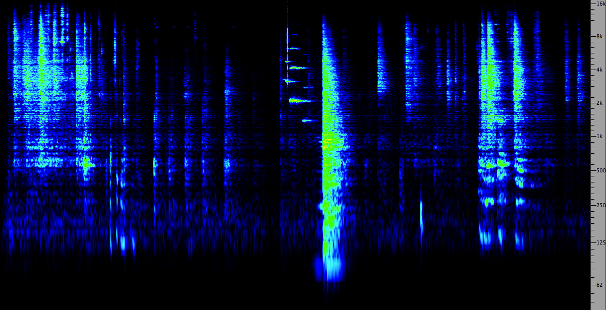
Another effect of convolution with Impulse
Reverb is the smearing of attacks, as shown below. This
effect occurs with reverberation because of the early
reflections combining with the original sound. It is often
not very noticeable, as we saw in the first sound example
where we compared digital algorithmic reverb with impulse
reverb. The algorithmic reverb minimized this smearing and
kept the attack stronger, and seemingly closer. With auto-convolution (convolving
the sound with itself) attacks are almost completely gone.

Smearing
of
attacks in impulse reverb
However, what if we wanted to change a steady broadband
sound into a percussive one - could we use an IR to do
that? The answer is "yes", but we would have to use a
Moving Window in the Convolution process (which not all
Convolution software includes), so that the source sound
is progressively convolved with just a short amount amount
of the IR, starting at the beginning, then moving to the
next window and so on. The shorter the window, the more
compact the attack will be and the less amplitude the
decay will have. The advantage over applying a simple
amplitude envelope is that the spectrum will decay more
like an echo than a simple fade-out. Note that the
Brighten option wasn't used in these examples to boost the
high frequencies.
Source: Squeaky train sounds
|
Impulse response of a Turrell
Skyspace
|
without a Moving Window
|
with a 1 sec. Moving Window
|
with a .5 sec. Moving Window
|
with a .25 sec. Moving Window
|
with a .1 sec. Moving Window
|
Index
C. Studio Demo of Reverberation. Reverberation
in studio production is usually added within the context
of a mix, particularly if plug-ins are being used. In
the previous section, we raised the possibility of using
Impulse Reverb as a means of processing individual
sounds, presumably prior to being used in a mix, or as
in the dry/wet example of Prospero’s speech,
incorporating each version within a subsequent mix.
In
both analog and digital mixing contexts, the Auxiliary
circuit has been and still is the standard way
to incorporate reverberation into a mix with each
track given the option of whether it is reverberated,
and if so, with what strength and characteristics. We
have already encountered the Auxiliary circuit in the
design of parallel
processing, where a signal can be sent to
multiple processors via multiple auxiliaries.
Here we use the more traditional route of using one
Aux circuit to send multiple signals to the same
processor, in this case a reverberator, as shown
in this diagram.

In an analog mixer, each input channel has the
option of sending the signal directly to an output channel
AND sending it to one or more Auxiliary circuits with a
level that is independent of the signal level going to the
output channel. We’ll call these the mix level and
the Aux send level, respectively. In other words,
what this creates is a kind of submix, where all
signals going to the same Auxiliary channel are mixed
together with their own relative strengths, independent of
what is going into the final mix itself.
The other, very important choice is the
relationship between the mix level and the Aux send level,
the choices always referred to as pre or post.
These terms are short for pre-fader and post-fader.
The distinction is:
- the “pre” setting sends the signal independent
of the mix level, i.e. “before” that level, hence the
use of “pre”
- the
“post” setting sends the signal that is dependent
on the mix level, i.e. “after” that level, hence the use
of “post”
The Aux
send level is going to a processor, such as a
reverberator, and then it returns to the overall mix via
the Aux return (which you can Solo, in
order to hear it alone for fine adjustment). The Aux
return level in the mix has its own fader to control how
much global reverb goes into the mix. Therefore,
we have two situations:
- in the “pre” setting, the processed
signal always goes to the mix whether the
original signal is there or not; this is useful for
making the sound move into the distance, for instance,
as described above in terms of the dry/wet mix
- in
the “post” setting, the processed signal only
goes to the mix when the original signal is there too,
so fading out the original signal means fading out the
reverb, in this case; this is likely to be the more
usual situation
Mix demo. Here is a typical mix
configuration with three stereo tracks on channels 14, 15
and 16. On each of those tracks, Aux A (or 1) has a Send
activated. In the case of ProTools, only one of these is
shown at a time, so this diagram has been photoshopped to
include all three, just so you can see that they all have
“post” selected (by not selecting “pre”). Each
track has its own Send Level (which will control the
signal level of each track being sent to the
reverberator), and each Aux Send is going to a particular
output “bus” (which is basically a virtual patch cord that
connects the signal to the Aux channel shown to the right
of the signal channels.
This Aux channel (highlighted in the bottom right corner),
which receives its signal from the same bus, has an insert
selected, which is the stereo DVerb plug-in. Its output
goes into the overall mix (channels 1&2). Check that
you understand the routing involved by enlarging the
diagram and using the zoom tool if necessary.
Note that if the DAW software (stupidly) labels the output
as going to a specific processor (in this case, a
compressor), you can ignore this and add the processor of
your choice as an Insert. Don't let yourself be "dumbed
down"!
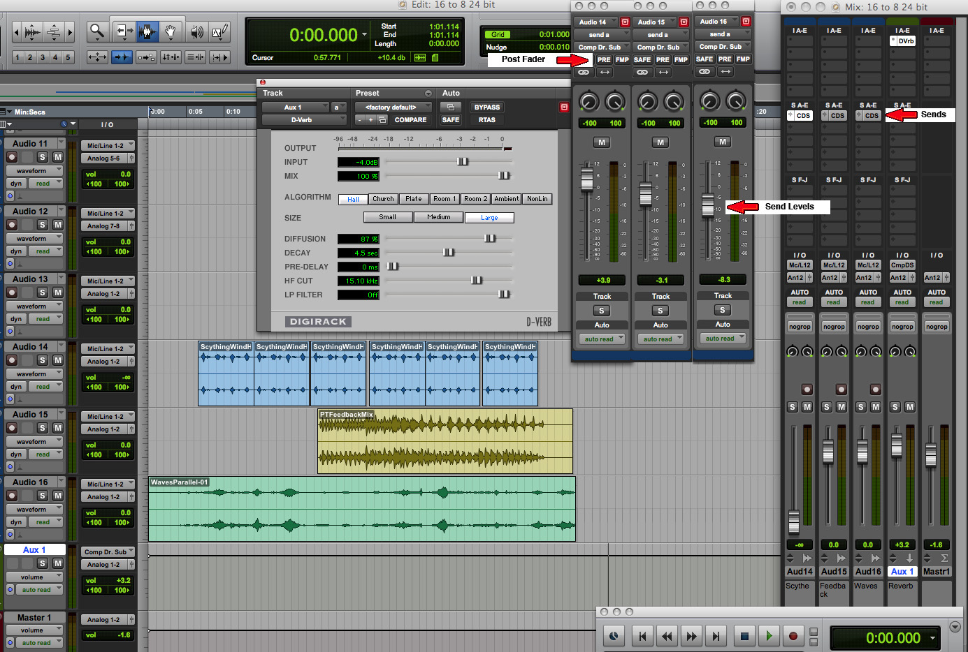
Three source mix with reverb (Click to enlarge)
This
demo mix uses three soundfiles we have generated in
previous exercises, ones that actually don’t make much
logical sense in combination: (1) the high-pass scything
sound; (2) the feedback circuit mix that combines rhythmic
hammering with the percussive PVC pipe; (3) the mix of
waves used in the parallel circuit. However, we accept the
challenge of trying to make “aural” sense of these three
semantically unrelated sounds.
Moreover, why would anyone want to put reverb on the
scythe and the waves? They clearly are not going to be
recognized as belonging to the same acoustic space! But
they both do have rhythmic noisy timbres, so we can play
on that.
There are three versions of our mix: (1) no reverb, so the
illogical elements stay quite separate; (2) a mix with 4.5
seconds of reverb, but note that each Aux send has a
different level, more going to the scythe, medium going to
the rhythmic mix, and less going to the waves; (3) we
raise the reverb level by a factor of more than 2 to about
10 seconds. You may also notice that a bit of care has
been taken in placing the rhythmic repetitions of the
scythe against the rhythms of the feedback circuit and the
waves.
Mix with no reverb
Mix with medium reverb
Mix with high reverb
|
Click to enlarge
|
In
these mixes, no attempt was made to adjust the mix levels
(at least not yet, stay tuned), except for a simple
fade-in and out at each end. How did you find the balance
of the elements? Which version did you prefer? Despite the
illogical nature of the mix from a semantic perspective, I
think mix 2 is the best, because the reverb, however,
incongruent, helps to blend the three tracks into a unity,
supports the build-up of rhythmic energy towards the end,
and still allows individual tracks to be heard clearly.
Mix 3 is “swimming” in reverb, and possibly drowning the
component sounds. Think of the balance between envelopment
and definition referred to earlier – this mix skews the
balance towards envelopment at the expense of clarity.
Auxiliary send in Pre mode. Here
is a simple example of how to make the sound appear to
recede in the distance by simply fading out the unmodified
signal, while keeping a constant level of reverb. As
described above, the “pre” setting allows this to be
easily accomplished. In the example the mix level has been
latched to fade out (doing this by ear is a good idea,
instead of using breakpoints).
The single Aux circuit is in pre mode, and the
send level is at 0 dB. The Dverb is set to “large church”,
similar to the convolved version heard earlier, with a 8.7
sec reverb time. It would be a bit more accurate in terms
of how this works in the real world, to slowly attenuate
the reverb level as well, but much more slowly, on the Aux
return (which can also be latched).
The principle here is that in an acoustic space, the
direct signal from the source falls off at 6 dB per
doubling of distance (the inverse-square
law), but the reverberated portion falls off much
more slowly so that the ratio of dry/wet gradually
favours a larger percentage of the sound being the
reverberated portion.

Click to enlarge
|
Voice appearing to recede
|
Index
D. Studio demo of Impulse Reverb.
Most app’s that offer Impulse Reverb or Convolution Reverb
have a simple set of parameters, including the wet/dry
mix which avoids having to use multiple IR files
recorded at different distances. Also, look for a pre-delay
option, and the type of EQ or filtering that is
offered. Some app’s provide an extensive catalogue of
Impulse Responses, and the option of importing others.
However, if the software doesn't allow the reverb process
to be extended to auto-convolution, or any other arbitrary
combination of files, it is going to be limited in terms
of what we are developing here.
However, keep in mind, that you may have to add several
seconds of silence to your file if you don’t want
to have it cut off once you apply it to your sound – a
typical demonstration of how inflexible the processing
paradigm is, despite the obvious need to incorporate this
into your processing. This problem will likely be true of
DAW’s as well as editors.

"ImpulseVerb" in the Peak editor
Some editors may also allow you to use the “impulse” from
the clipboard. This means you load the IR (or the
file itself for auto-convolution) into the editor first,
copy it to the clipboard (command C), and then use it for
the Impulse Reverb. Since auto-convolution doubles the
length of the output file, you will need to add that much
silence to the soundfile, all of which makes one
appreciate SoundHack more, since its author, Tom Erbe,
obviously knows what is really involved with convolution.
With SoundHack, Impulse Reverb is a typical process of
loading the source file (command O), selecting Convolution
from the Hack menu (command C), at which point your file
will be labelled “Input”, then you can add Normalization
and (optionally) Brighten, and select the Impulse File,
which is then labelled as “Impulse”.

SoundHack
Convolution
At this point you’re ready to process the file, giving it
a more compact name than the suggested one, and choosing 24
bit output. You can test it out by playing it in the
bar at the bottom, but if you want to edit it, delete the
file from SoundHack on the desktop, and open the file in
your editor (i.e. you can't have two versions of the
output file open at the same time). As noted above, if you
want to further move your sound around in the space you've
created, multi-track the original with this processed
version and adjust levels and panning.
Note: SoundHack convolution will only work with .aif files
(not .wav) on the Mac.
Index
Q. Try
this review quiz
to test your comprehension of the above material,
and perhaps to clarify some distinctions you may
have missed.
home
