Postscript version of this file

STAT 870 Lecture 9

strong Markov property:

Stopping time for the Markov chain is a random variable T taking values in $\{0, 1,\cdots\}\cup\{\infty\}$ such that for each finite k there is a function f_k such that

$$1(T=k) = f_k(X_0,\ldots,X_k)$$

Notice that T_k in theorem is a stopping time.

Standard shorthand notation: by

P^x(A)

we mean

$$P(A\vert X_0=x) \, .$$

Similarly we define

$${\rm E}^x(Y)= {\rm E}(Y\vert X_0=x) \, .$$

Goal: explain and prove

$${\rm E}(f(X_{T},\ldots)\vert X_T,\ldots,X_0) = {\rm E}^{X_T}(f(X_0,\ldots))$$

Simpler claim:

$$P(X_{T+1}=j\vert X_{T}=i) = {\bf P}_{ij} = P^i(X_1=j) \, .$$

Notation: $A_k=\{X_{k}=i,T=k\}$

Notice: $A_k=\{X_T=k,T=k\}$:
$$\begin{align*}P(& X_{T+1}=j\vert X_{T}=i) = \frac{ P(X_{T+1}=j,X_{T}=i)}{P(X_T=i... ... P(X_{1}=j\vert X_{0}=i)P(A_k)}{\sum_k P(A_k)} \\ & ={\bf P}_{i,j} \end{align*}$$
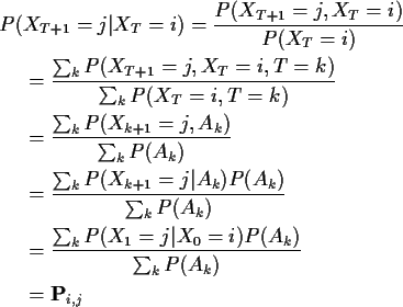
Notice use of fact that T=k is event defined in terms of $X_0,\ldots,X_k$.

Technical problems with proof:

$\bullet$ It might be that $P(T=\infty)>0$. What are X_T and X_T+1 on the event $T=\infty$.

Answer: condition also on $T<\infty$.

$\bullet$ Prove formula only for stopping times where $\{T < \infty\}\cap \{X_T=i\}$ has positive probability.

We will now fix up these technical details.

Conditional distributions, expectations

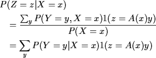
When X and Y are discrete we have

$${\rm E}(Y\vert X=x) = \sum_y P(Y=y\vert X=x)$$

for any x for which P(X=x) is positive.

Defines a function of x.

This function evaluated at X gives rv which is ftn of X denoted

$${\rm E}(Y\vert X) \, .$$

Here are some properties of that function.

1)

Suppose A is a function defined on the range of X. Then

$${\rm E}(A(X)Y\vert X=x) = A(x){\rm E}(Y\vert X=x)$$

and so

$${\rm E}(A(X)Y\vert X) = A(X){\rm E}(Y\vert X)$$

Second assertion follows from first. Note that if Z=A(X) Y then Z is discrete and

$$P(Z=z) = \sum_{x,y} P(Y=y,X=x) 1( z = A(x) y)$$

Also
$$\begin{align*}P&(Z=z\vert X=x) \\ & = \frac{\sum_y P(Y=y, X=x) 1(z=A(x)y)}{P(X=x) } \\ & = \sum_y P(Y=y\vert X=x)1(z=A(x)y) \end{align*}$$
Thus
$$\begin{align*}{\rm E}&(Z\vert X=x) \\ & =\sum_z z P(Z=z\vert X=x) \\ & = \sum... ...y\vert X=x) \sum_z 1(z=A(x)y) \\ & = A(x) \sum_y yP(Y=y\vert X=x) \end{align*}$$

2)

Repeated conditioning: if X, Y and Z discrete then
$$\begin{align*}{\rm E}\left\{{\rm E}(Z\vert X,Y)\vert X\right\} & = {\rm E}(Z\vert X) \\ {\rm E}\left\{{\rm E}(Y\vert X)\right\} & = {\rm E}(Y) \end{align*}$$

3)

Additivity

$${\rm E}(Y+Z\vert X)={\rm E}(Y\vert X)+{\rm E}(Z\vert X)$$

4)

Putting the first two items together gives

$${\rm E}\left\{{\rm E}(A(X)Y\vert X) \right\} {\rm E}(A(X)Y)$$ (1)

Definition of ${\rm E}(Y\vert X)$ when X and Y are not assumed to discrete:

${\rm E}(Y\vert X)$ is rv which is measurable function of X satisfying(1).

Existence is measure theory problem.

Suppose $f(x_0,x_1,\ldots)$ is a (measurable) function on $S^{\Bbb N}$. Put

$$Y_n = f(X_n,X_{n+1},\ldots)\, .$$

Assume ${\rm E}(\, \vert Y_0\vert \, \vert X_0=x)<\infty$ for all x. Claim:

$${\rm E}(Y_n\vert X_n,A) = {\rm E}^{X_n}(Y_0)$$ (2)

whenever A is any event defined in terms of $X_0,\ldots,X_n$.

Proof:

• Family of f for which claim is true includes all indicators; see extension of Markvo Property in previous lecture.

• family of f for which claim is true is vector space (so if f, g in family then so is af+bg for any constants a and b.

• So family of f for which claim is true includes all simple functions.

• family of f for which claim true is closed under monotone increasing limits (of non-negative f_n) by the Monotone Convergence theorem.

• So claim true for every non-negative integrable f.

• Claim follows for integrable f by linearity.

Aside on ``measurable'': what sorts of events can be defined in terms of a family $\{Y_i: i \in I\}$?

Natural: any event of form $(Y_{i_1}, \ldots, Y_{i_k}) \in C$is ``defined in terms of the family'' for any finite set $i_1,\ldots,i_k$and any (Borel) set C in S^k.

For countable S: each singleton $(s_1,\ldots,s_k)\in S^k$ Borel. So every subset of S^k Borel.

Natural: if you can define each of a sequence of events A_n in terms of the Ys then the definition ``there exists an n such that (definition of A_n) ...'' defines $\cup A_n$.

Natural: if A is definable in terms of the Ys then A^c can be defined from the Ys by just inserting the phrase ``It is not true that'' in front of the definition of A.

So family of events definable in terms of the family $\{Y_i: i \in I\}$ is a $\sigma$-field which includes every event of the form $(Y_{i_1}, \ldots, Y_{i_k}) \in C$. We call the smallest such $\sigma$-field, ${\cal F}(\{Y_i: i \in I\})$, the $\sigma$-field generated by the family $\{Y_i: i \in I\}$.

This discussion permits some shorthand. We define

$${\cal F}_n = {\cal F}(\{X_0,\ldots,X_n\})$$

and

$${\cal F}_\infty = {\cal F}_(\{X_0,X_1,\ldots\})$$

Conditioning on $X_0,\ldots,X_T$ where T is a stopping time?

Method 1: regard vector $X_0,\ldots,X_T$ as taking values in exotic space, namely:

$$\left(\bigcup_{n=1}^\infty S^n \right) \bigcup S^{\Bbb N}$$

We define

$${\cal F}_T = {\cal F}(X_0,\ldots,X_T)$$

Random vector $X_0,\ldots,X_T$ is discrete on $T<\infty$ but not discrete on $T=\infty$.

Suppose X is discrete and X^*=g(X) is a one to one transformation of X. Since X=x is the same event as X^*=g(x) we find

$${\rm E}(Y\vert X=x) = {\rm E}(Y\vert X^*=g(x))$$

Let h^*(u) denote the function ${\rm E}(Y\vert X^*=u)$ and $h(u)={\rm E}(Y\vert X=u)$. Then

h(x)=h^*(g(x))

Thus

h(X) = h^*(g(X)) = h^*(X^*)

This just means

$${\rm E}(Y\vert X)= {\rm E}(Y\vert X^*)$$

Interpretation.

Formula is ``obvious''.

Example: Toss coin n=20 times. Y is indicator of first toss is a heads. X is number of heads and X^* number of tails. Formula says:

$${\rm E}(Y\vert X=17) = {\rm E}(Y\vert X^*=3)$$

In fact for a general k and n

$${\rm E}(Y\vert X=k) = \frac{k}{n}$$

so

$${\rm E}(Y\vert X) = \frac{X}{n}$$

At the same time

$${\rm E}(Y\vert X^*=j) = \frac{n-j}{n}$$

so

$${\rm E}(Y\vert X^*) = \frac{n-X^*}{n}$$

But of course X=n-X^* so these are just two ways of describing the same random variable.

Another interpretation: Rv X partitions $\Omega$ into countable set of events of the form X=x.

Other rv X^* partitions $\Omega$ into the same events.

Then values of ${\rm E}(Y\vert X^*=x^*)$ are same as values of ${\rm E}(Y\vert X=x)$ but labelled differently.

To form ${\rm E}(Y\vert X)$ take value $\omega$, compute $X(\omega)$ to determine member A of the partition we being conditionsed on, then write down corresponding ${\rm E}(Y\vert A)$.

Hence conditional expectation depends only on partition of $\Omega$.

X not discrete: replace partition with $\sigma$-field. Suppose X and X^* 2 rvs such that ${\cal F}(X) = {\cal F}(X^*)$. Then:

• There is g Borel,one to one with one to one Borel inverse s.t. X^*=g(X).

• ${\rm E}(Y\vert X)={\rm E}(Y\vert X^*)$ almost surely.

In other words ${\rm E}(Y\vert X)$ depends only on the $\sigma$-field generated by X. We write

$${\rm E}(Y\vert{\cal F}(X))={\rm E}(Y\vert X)$$

Definition: Suppose ${\cal G}$ is sub-$\sigma$-field of ${\cal F}$. X is ${\cal G}$ measurable if, for every Borel B

$$\{\omega: X(\omega) \in B\} \in {\cal G} \, .$$

Definition: ${\rm E}(Y\vert{\cal G})$ is any ${\cal G}$ measurable rv s.t.  for every ${\cal G}$ measurable rv variable Awe have

$${\rm E}(AY) = {\rm E}\left\{A{\rm E}(Y\vert{\cal G})\right\} \, .$$

Again existence is measure theory problem.

Now we define ${\cal F}_T$ to be the collection of all events B such that

$$B\cap \{T \le n\} \in {\cal F}_n$$

for each n. It is easy to prove that ${\cal F}_T$ is a $\sigma$-field and that T and X_T are ${\cal F}_T$measurable.

Rewrite Strong Markov Property: if

• $f:S^{\Bbb N} \mapsto {\Bbb R}$ is Borel and

• $Y_T = f(X_T,X_{T+1}, \ldots)1(T<\infty)$ and

• $Y_0 = f(X_0,X_1,\ldots)$ and

• ${\rm E}^x(\vert Y_0\vert) < \infty$ for all x.

then
$$\begin{multline*}1(T<\infty){\rm E}(f(X_{T},X_{T+1},\ldots)\vert{\cal F}_T) \\ = 1(T<\infty){\rm E}^{X_T}(f(X_0,X_1,\ldots)) \end{multline*}$$

Proof of Strong Markov Property.

Since T is ${\cal F}_T$ measurable we have
$$\begin{multline*}1(T<\infty){\rm E}\left\{f(X_{T},X_{T+1},\ldots)\vert{\cal F}_T... ...left\{ 1(T<\infty)f(X_{T},X_{T+1},\ldots)\vert{\cal F}_T\right\} \end{multline*}$$
Suppose A is ${\cal F}_T$ measurable; need only prove
$$\begin{multline*}{\rm E}\left[A1(T<\infty){\rm E}^{X_T}\left\{f(X_0,X_1,\ldots)\... ... \\ = {\rm E}\left\{A1(T<\infty)f(X_{T},X_{T+1},\ldots)\right\} \end{multline*}$$

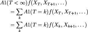
Break up the events according to value of T:
 $$\begin{align*} A1(T< &\infty) {\rm E}^{X_T}\left\{f(X_0,X_1,\ldots)\right\} \\ ... ...\\ & = \sum_k A1(T=k){\rm E}^{X_k}\left\{f(X_0,X_1,\ldots)\right\} \end{align*}$$

On the other hand
$$\begin{align*}A1(&T<\infty)f(X_{T},X_{T+1},\ldots) \\ & = \sum_k A1(T=k)f(X_{T},X_{T+1},\ldots) \\ & = \sum_k A1(T=k)f(X_k,X_{k+1},\ldots) \end{align*}$$
But by our extended Markov property
$$\begin{align*}{\rm E}& \left\{ A1(T=k)f(X_k,X_{k+1},\ldots)\right\} \\ & = {\r... ...\left[A1(T=k){\rm E}^{X_k}\left\{f(X_0,X_{1},\ldots)\right\}\right] \end{align*}$$
Exactly expectation of kth term in (). This proves the Strong Markov Property.