Methodology
How it's done
Our objective is to compare perceived walkability and objective walkability in three neighborhoods. To do this we will create an objective walkability surface and a perceived walkability surface for each neighborhood and then compare the two. A surface, or field, has been chosen to represent walkability rather than an object as it better represents the continuous nature of the phenomena. Walkability does not end at an arbitrarily defined neighborhood boundary and it is not limited to a single point. As well, walkability is not evenly distributed throughout the spatial object that represents a neighborhood and is therefore better represented as a field. As the project progresses, two methodological issues will need to be addressed: what spatial scales are appropriate for meeting different needs and at what spatial scale or level of aggregation is information actually available (Macintyre, Elleway, and Cummin, 2002, 134-135)? Preliminary methods for constructing each walkability surface are described below.
Objective Walkability
The factors of land use mix, dwelling density, and connectivity are not directly available through the Open Data Catalogue in analysis ready form. They must be derived from other sources such as street networks and building footprints represented as vector data. The factors are derived as either a density or a ratio that is then used to create raster layers for the neighborhoods. The layers are then combined to create the final walkability surface. How each factor was derived, normalized and then combined to create the final objective walkability surface for each neighbourhood is described below.
Street Connectivity was determined using a point density analysis. Only Vancouver city streets were considered when measuring connectivity; highways, private roads, and lanes were excluded from the analysis. Intersections were marked as a point. Only intersections connecting three or more streets were marked (Leslie et al 2007, 116; Frank et al 2010, 925). Examples of street connections are provided below:
 Once marked, a point density analysis was used to create a surface for the neighbourhood. The analysis counted all points within a square kilometer of the center
of the raster grid cell. The square kilometer was defined by
a square 1000m on each side. A square search area rather than a circle of radius 564m was chosen as this better reflected the grid pattern of the street network.
Dwelling Density was also measured with a point pattern analysis. All residentially zoned properties were marked as a point. A point density analysis was then used to create the dwelling density surface. Again, a square search area with an area of 1km2 was used for the analysis to maintain consistency with the street connectivity surface.
Land Use Mix was determined based on the equation used by Frank et al (2005, 117) and Leslie et al (2007, 116) where k is the category of land use; p is the proportion of the land area devoted to a specific land use; N is the number of land use categories:
Once marked, a point density analysis was used to create a surface for the neighbourhood. The analysis counted all points within a square kilometer of the center
of the raster grid cell. The square kilometer was defined by
a square 1000m on each side. A square search area rather than a circle of radius 564m was chosen as this better reflected the grid pattern of the street network.
Dwelling Density was also measured with a point pattern analysis. All residentially zoned properties were marked as a point. A point density analysis was then used to create the dwelling density surface. Again, a square search area with an area of 1km2 was used for the analysis to maintain consistency with the street connectivity surface.
Land Use Mix was determined based on the equation used by Frank et al (2005, 117) and Leslie et al (2007, 116) where k is the category of land use; p is the proportion of the land area devoted to a specific land use; N is the number of land use categories:
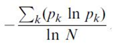 Four of the land use categories were used to determine land use mix in this study: residential, commercial, industrial, and institutional. The City of Vancouver identifies some properties as properties as mixed residential and commercial. In this case the property was counted as part of both categories. Land use mix was then calculated as a single score, between 0 and 1, for each neighborhood.
To conform to the standards of the land use mix score the values for the two surfaces were standardized across all three neighbourhoods to a score between 0 and 1 with the equation:
Standard= (V-Vmin)/(Vmax-Vmin)
Where V is the measured variable.
The final walkability surface was created by combining the dwelling density and street connectivity surfaces along with the land use score separately for each neighbourhood by the formula described by Frank et al (2010, 925):
Walkability=(2*Street Connectivity)+(Dwelling Density)+(Land Use Mix)
Four of the land use categories were used to determine land use mix in this study: residential, commercial, industrial, and institutional. The City of Vancouver identifies some properties as properties as mixed residential and commercial. In this case the property was counted as part of both categories. Land use mix was then calculated as a single score, between 0 and 1, for each neighborhood.
To conform to the standards of the land use mix score the values for the two surfaces were standardized across all three neighbourhoods to a score between 0 and 1 with the equation:
Standard= (V-Vmin)/(Vmax-Vmin)
Where V is the measured variable.
The final walkability surface was created by combining the dwelling density and street connectivity surfaces along with the land use score separately for each neighbourhood by the formula described by Frank et al (2010, 925):
Walkability=(2*Street Connectivity)+(Dwelling Density)+(Land Use Mix)
Perceived Walkability
Scans provide additional benefits beyond time and ethics; they also provide a measure of control over how the questions are answered. Questionnaires completed by participants require the respondents to first interpret the questions and then decide on a satisfactory answer. The researchers must then in turn interpret the participant’s qualitative responses, increasing the possibility of miscommunication.
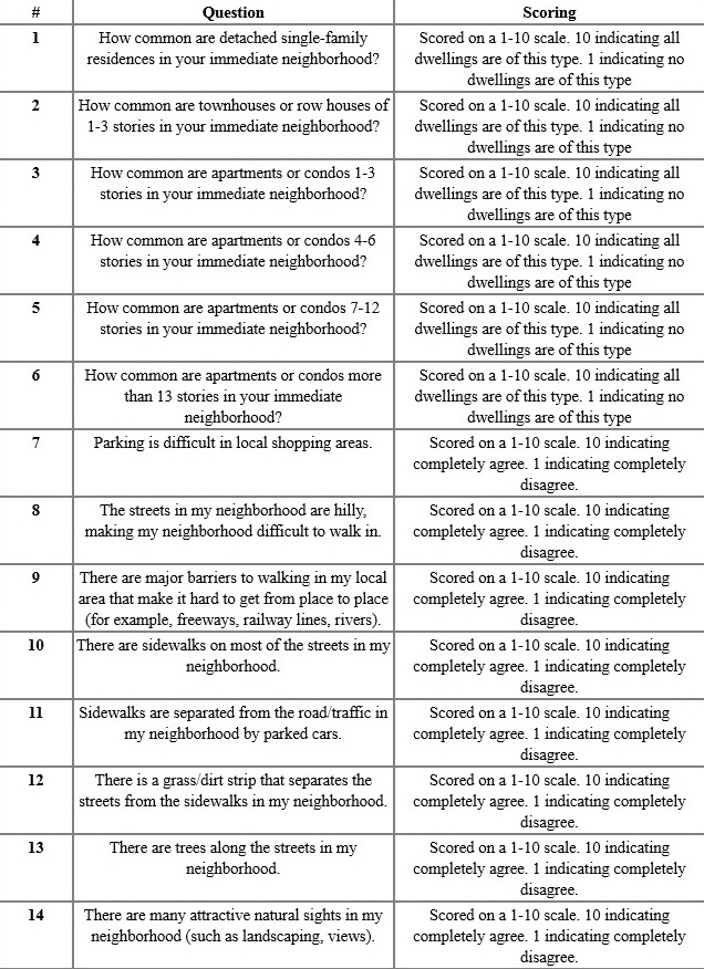
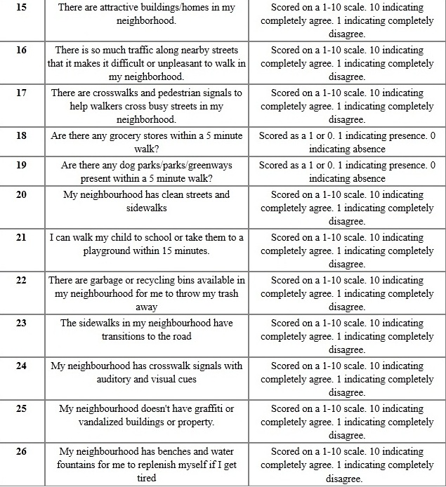
The conversion of the NEWS-A questionnaire to a scan criterion involved removing questions that required specific local knowledge. An example of such a question is, can walkers and bikers on the streets in my neighborhood be easily seen by people in their homes (NEWS-A, 6)? In addition, all of section B of the NEWS-A questionnaire was removed. Section B is comprised of questions about perceived distance. Respondents provide estimated walking times to a list of locations. These times are then converted to distance based on an average walking speed. Not only would this be difficult for the researchers to answer, but it has been noted as a problematic section of the questionnaire (McCormack et al 2007, 19-21). The conversion of time estimates to distances involves a great amount of uncertainty. The scan criteria and scoring system is outlined below:
 To create a single walk score the question responses were combined in the following manner. Questions 1-6 were amalgamated to a single residential density score as per the NEWS scoring procedures (2002) for calculating residential desnity. The following equation was used:
RD=(Question 1 Score)/2+(12*(Question 2 Score)/2)+(10*(Question 3 Score)/2)+(25*(Question 4 Score)/2)+(50*(Question 5 Score)/2)+(75* (Question 6 Score)/2)
The Residential Density scores were then standardized to a 1 to 10 scale. Questions 7, 8, and 9 were phrased in such a way that a score of 10 indicated poor walkability characteristics. Consequently these questions had their scores reversed with 10 reversed to a 1, 9 reversed to a 2, and so on. The standardized residential density and the reversed scores were then added together with the raw scores from every other question to produce a single walkability score for each location, with the maximum possible score being 192 and the lowest possible score being 19. Of the 36 total sample points across the three neighbourhoods the highest actual score was 146 and the lowest was 75.
The conversion to scans does create some limitations. Most notably, whose perception is being measured? The perceptions of the project members may not reflect the perceptions of the neighborhood given that we do not form a representative sample; there being only four members all of similar age and socioeconomic status (university undergraduates). However, for the goals and timeline of this project the conversion to scans is considered necessary.
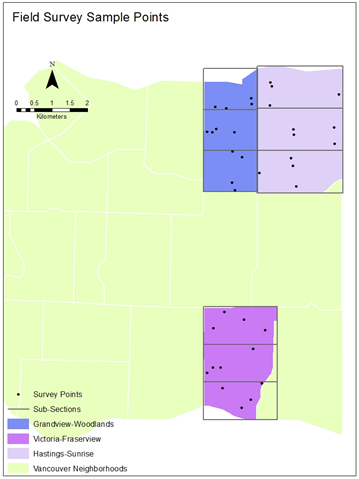
Scans were conducted at 12 sampling locations in each neighborhood. A stratified random sampling method will be used to select the sampling locations. Each neighborhood is split into three sections: north, central, and south. Each section has an approximately equal north-south distance. However, the area of each section is not the same due to the irregular shape of the neighborhoods. Four sampling locations based on address information in each section were randomly selected for scans. Survey locations are shown here:
To create a single walk score the question responses were combined in the following manner. Questions 1-6 were amalgamated to a single residential density score as per the NEWS scoring procedures (2002) for calculating residential desnity. The following equation was used:
RD=(Question 1 Score)/2+(12*(Question 2 Score)/2)+(10*(Question 3 Score)/2)+(25*(Question 4 Score)/2)+(50*(Question 5 Score)/2)+(75* (Question 6 Score)/2)
The Residential Density scores were then standardized to a 1 to 10 scale. Questions 7, 8, and 9 were phrased in such a way that a score of 10 indicated poor walkability characteristics. Consequently these questions had their scores reversed with 10 reversed to a 1, 9 reversed to a 2, and so on. The standardized residential density and the reversed scores were then added together with the raw scores from every other question to produce a single walkability score for each location, with the maximum possible score being 192 and the lowest possible score being 19. Of the 36 total sample points across the three neighbourhoods the highest actual score was 146 and the lowest was 75.
The conversion to scans does create some limitations. Most notably, whose perception is being measured? The perceptions of the project members may not reflect the perceptions of the neighborhood given that we do not form a representative sample; there being only four members all of similar age and socioeconomic status (university undergraduates). However, for the goals and timeline of this project the conversion to scans is considered necessary.
Scans were conducted at 12 sampling locations in each neighborhood. A stratified random sampling method will be used to select the sampling locations. Each neighborhood is split into three sections: north, central, and south. Each section has an approximately equal north-south distance. However, the area of each section is not the same due to the irregular shape of the neighborhoods. Four sampling locations based on address information in each section were randomly selected for scans. Survey locations are shown here:
 After the scans were completed walkability scores were calculated for each point. The point attributes were then be converted to a field through interpolation by kriging. Inverse distance weighting was considered as it allows for more control over the influence of distance. Some studies do provide estimates for the influence of distance on walkability (McCormack et al, 2007), however considering the group members’ limited expertise on walkability kriging was chosen as the interpolation method. The Kriging method of interpolation relies on an auto generated semivariogram to determine the influence of distance and the results of which may be beneficial to this project. The semivariogram determines the influence of distance by comparing the spatial variability and attribute variability of the sample points. The semivariogram also determines a distance at which points no longer exert any influence over their neighbors.
In the selection of sampling points it is recognized by the researchers that any sampling method chosen will be subject to the Modifiable Unit Area Problem. Were a different sampling method, sectioning method, or neighborhood boundary definition used the results of this project will be affected. The north, central, and south section classification method was chosen due to the long north-south axis of all three neighborhoods and their proximity to the water where the neighborhoods become increasingly more industrialized. A completely random sampling method was considered, but a stratified random sampling method was chosen as it ensured that the sample points would be dispersed throughout the neighborhoods.
After the scans were completed walkability scores were calculated for each point. The point attributes were then be converted to a field through interpolation by kriging. Inverse distance weighting was considered as it allows for more control over the influence of distance. Some studies do provide estimates for the influence of distance on walkability (McCormack et al, 2007), however considering the group members’ limited expertise on walkability kriging was chosen as the interpolation method. The Kriging method of interpolation relies on an auto generated semivariogram to determine the influence of distance and the results of which may be beneficial to this project. The semivariogram determines the influence of distance by comparing the spatial variability and attribute variability of the sample points. The semivariogram also determines a distance at which points no longer exert any influence over their neighbors.
In the selection of sampling points it is recognized by the researchers that any sampling method chosen will be subject to the Modifiable Unit Area Problem. Were a different sampling method, sectioning method, or neighborhood boundary definition used the results of this project will be affected. The north, central, and south section classification method was chosen due to the long north-south axis of all three neighborhoods and their proximity to the water where the neighborhoods become increasingly more industrialized. A completely random sampling method was considered, but a stratified random sampling method was chosen as it ensured that the sample points would be dispersed throughout the neighborhoods.