Data Manipulation

PROCEDURES:

ArcGIS

           I imported the gvrd_2001_landuse vector shape file first to get the predifined Projected Coordinate System for the rest of the layers which was the "NAD 1983 UTM Zone 10N" and also the predifined Geographic Coordinate System which was the "North American Datum 1983". After that, I opened the attributes table and selected my attributes based on "name" and got the unique values in order to select 'City of Langley' so that all the attributes would be highlighted.

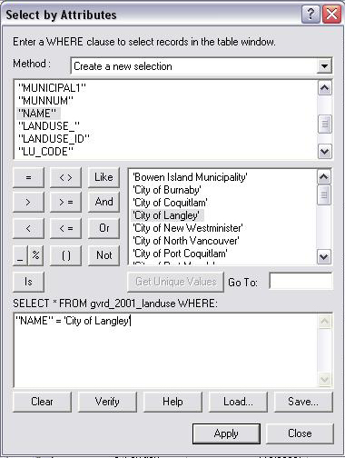
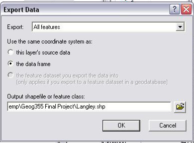
Digitizing the city of Langley out from te rest of the GVRD

         Since there was a piece of Langley missing, I had to switch the method to "add to current selection" and added the 'Township of Langley' as well. After this, all of Langley BC Canada was highlighted and I exported this data by "right clicking" on the "gvrd_2001_landuse layer" --> "data" --> "export data" and selected "all features in the data frame", thus creating my new shape file of Langley, BC Canada.

Exporting all of Langley into a new shape file

 
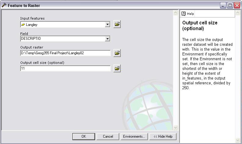
         Now that I have a vector shape file of Langley, I selected the properties and selected the "symbology tab" then "categories" for the "unique values" and selected "descriptio" in the "value field" and added all the values in order to get the land-use of Langley. After this, I had to turn this shape file into a raster file and in order to do this I had to open up "ArcToolbox" and look for "Conversion Tools" --> "To Raster" --> "Feature to Raster". Under the "input features" I selected Langley shape file, then under the "field" option I selected "DESCRIPTIO", the output file was named 'Langley' and the output cell size was set at "11". (What I realized was that any number can be entered, the default was 64 and the higher it is, the faster it will load in IDRISI. This was my mistake but I already had redone this step twice and it was too time consuming to switch back to 64. As long as you keep the cell size number consistent and the same for each shape file that you convert into raster, the whole model will work. If you don't do this, you will encounter "dimension" problems in IDRISI because the cell sizes for each shape to raster file are different) And so, this option converted the shape file into a raster file.

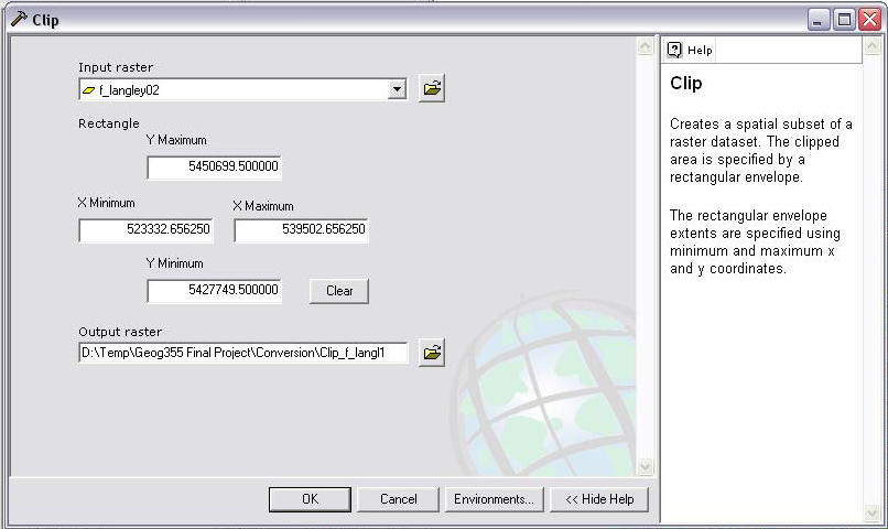
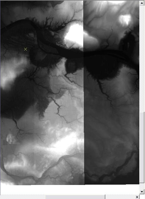
Converting feature shape file into raster format

         Now that you have a feature raster file, you can "clip" it so that the constraints will be all the same when you export to IDRISI. Under "Data Management Tools", you look for "Raster" --> "Clip" and select it. Since the land-use file was the biggest file, it will have the maximum boundaries for Langley and you have to copy down these minimum and maximums values for the X and Y axis's because these values will be the constraints for your other shape files that you decide to produce for your analysis. This picture shows my constraints so that all the dimensions for each raster file will be the same when exporting to IDRISI.

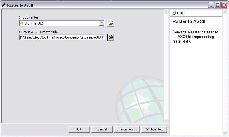
Clipping X and Y axis constraints of the raster file

          Finally the last procedure in exporting the raster file into IDRISI is selecting the "conversion tools"-->"from raster"-->"raster to ASCII" from "ArcToolbox". This is simple as you select the clip file and output it into ASCII raster file format. Your directories will get packed as you input more data and so to easily find these ASCII files in IDRISI, I labeled the output ASCII raster file as "ASCIILANGLEY.txt" so it is easy to find these files when using IDRISI.

Exporting raster file into ASCII format (To import into IDRISI)

          I added the "juststreets2" vector data in order to get my road network. This time I had to digitize it by selecting the roads within Langley, using the new Langley shape file that I created previously. After selecting all the roads within Langley, I exported it as a new shape file, naming it "Roads". The same steps previously mentioned were used in converting it to raster with the cell size "11" and clipping the road network using the same minimum and maximum values for the X and Y axis's and labeling it "ASCIIROADS.txt."

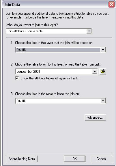
          The "disenumeration_areas.shp" vector data was added as well as the "census_bc_2001.dbf" file. I then used the "join" option in order to join the "census_bc_2001.dbf" to the "disenumeration_areas.shp" file using the DAUID as a reference in order for the information to be placed in the same polygon that is referenced to the same DAUID. So the DAUID works as a benchmark for all the information that could be added to same polygon or district as long as the information from each file contains the same DAUID.

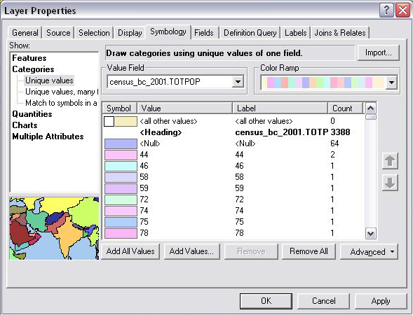
Joining of census data into disenumeration shape file using DAUID as the referencce

          After that, I had a disenumeration area of the whole GVRD in which digitizing had to be done in selecting only Langley. Once I had selected all the polygons I had to export it into a new shape file in which I called it "Disenumeration.shp". I then selected "total population" in "properties"-->"symbology"-->"cateogories"-->"unique values"-->"census_bc_2001.TOTPOP" in which it gave me different polygons with the different total population ranges.

Displaying the different total population ranges for each disenumeration area of Langley

          After this, I had to convert the feature to raster with the same cell size "11". And I then clipped it the same way and exported it into ASCII format calling it "ASCIIDISENUM.txt."

           The primary data that I collected which were the latitude and longitude data for the stores that sold pocket bikes was added to ArcGIS. I then selected the "Add XY Data" in which in the "X-axis field" was "LONG" for longitude and in the "Y-axis Field" it was "LAT" for latitude and the "spatial reference of input coordinates" required the "geographic coordinate system" of "North American Datum 1983.prj." And so, these points were added to my map and I had to export it as a shape file and repeat the whole process of feature to raster with the cell size of "11" and the clipping of the same axis's as the previous procedures. Finally it was exported raster to ascii labled as "ASCIISTORES.txt."

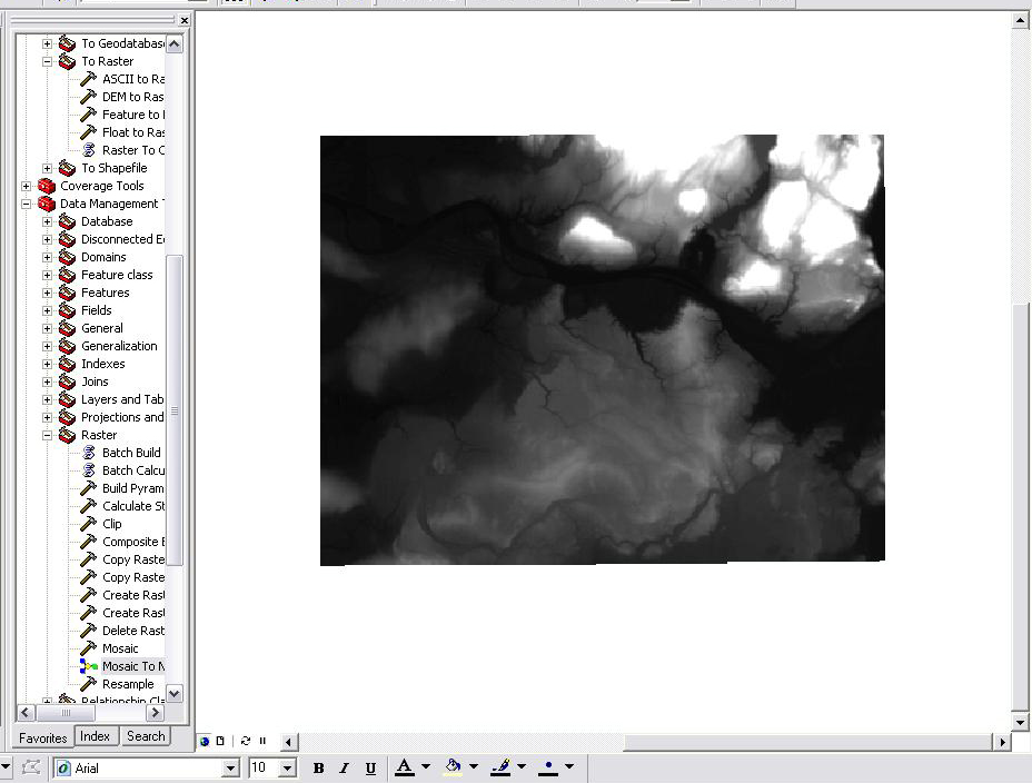
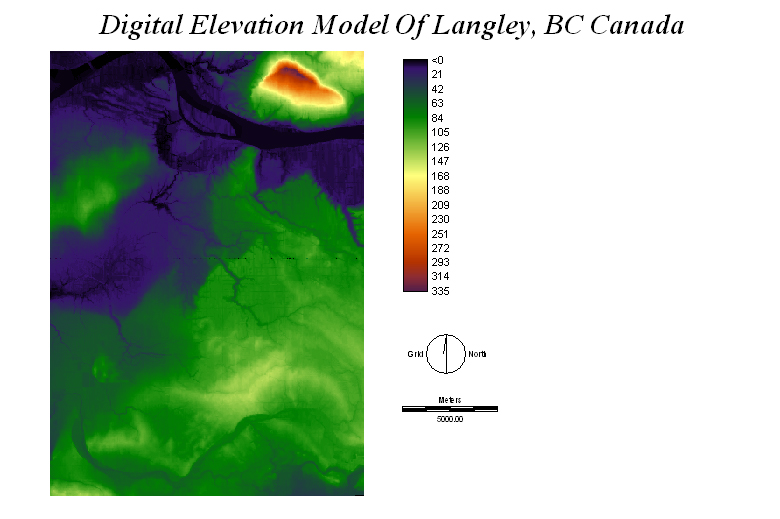
          Obtaining the DEM data was rather quite difficult for me to do. I had to find the data sets that covered Langley in which there were two data sets in which one data set covered a portion of Langley and the second data set covered the other portion of Langley. The data sets were "nts92g01e" and "nts92g01w" and in order to combine these data sets I had to look for "Mosaic to New Raster" under "Data Management Tools"-->"Raster"-->"Mosaic To New Raster" in "ArcToolbox."

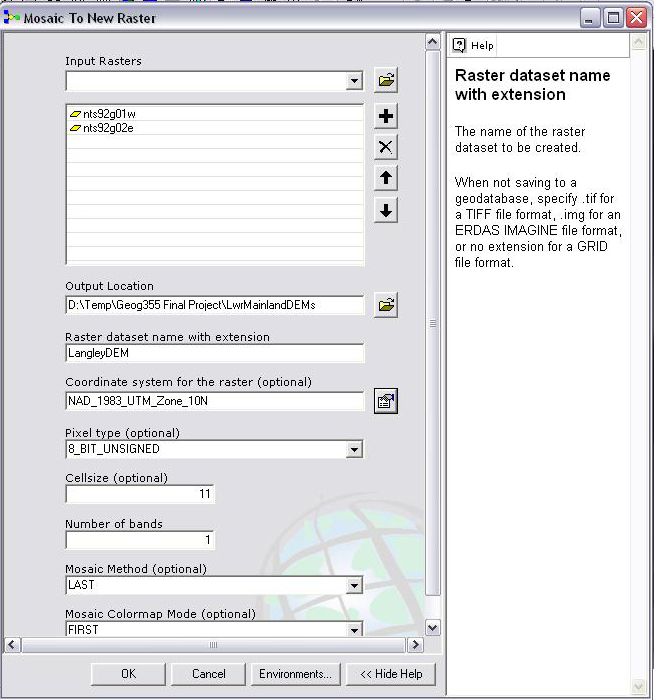
Using the Mosaic To New Raster tool in order to combine 2 DEMS that link up on the edges into one

          For the "input rasters" field I added the two datasets. Then I selected the "LwrMainlandDEM" folder in which to export the file, calling it "LangleyDEM". I then selected the "NAD_1983_UTM_Zone_10N" Projected Coordinate System with a cell size of "11". After all these steps, the two data sets were combined into one. The next step took me a while to figure out as I couldn't digitize the DEM areas that occur within Langley because there were so many different elevation values. And so, I clicked "properties" and under the "extent tab" I selected "set the extent to: the rectangular extent of langley" in which only the DEMs displayed the areas within Langley thanks to the previous shape files that I have worked on. All I had to do now was "clip" this "DEM mosaic" raster file since it is already in raster format. I then clipped it to the proper values for the X and Y axis's and then exported it to an ASCII file for IDRISI labeling it "ASCIIDEM.txt."

IDRISI Kilimanjaro

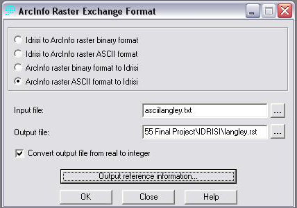
           In order to import these ASCII files, I had to go to "File"-->"Import"-->"Software-Specific Formats"-->"ESRI Formats"-->"ARCRASTER". By selecting ArcInfo raster ASCII format to IDRISI, I could locate the ASCII files that I created from ArcGis. For the "Input file", I selected "ASCIILANGLEY.txt" and for the "Output file", I named it "langley.rst." I then checked the "Convert output file from real to integer" box and left the "Output reference information" as default and pressed OK.

Importing ASCII into Idrisi raster format

           I repeated these steps for the other 4 ASCII files that I created in ArcGIS in order to import all these raster files into IDRISI raster file format.

Land-Use:
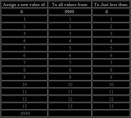
          After importing all these files, they all required to be "reclassed". For example the "langley landuse" raster file had a color range of <1 to 13 which indicated that there 13 land-use types plus the <1 indicated the null areas which were the areas outside of Langley, BC Canada such as the Fraser River.

My reclass file for Langley Landuse was:

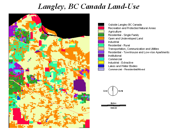
Reclassed Land-Use File of Langley, BC Canada

          In order to change these numbers into a proper legend, I had to select "Layer Properties" of the reclassed map and "view metadata"-->"legend" tab and manually add a legend to make it clearer of each of the different landuses for Langley. I had to compare the landuse in ArcGIS in order to make this legend for this raster file in IDRISI.

Land Constraint:

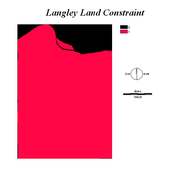
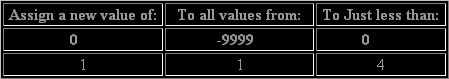
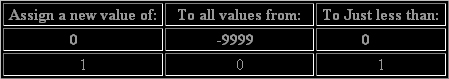
           After this, I reclassed the map and made a land constraint giving all the land use values a 1 and everything outside of Langley a value of 0. This was going to be one of my constraints as the shop has to be located any where within Langley.

Reclassed land-use for land constraint of all of Langley, BC Canada

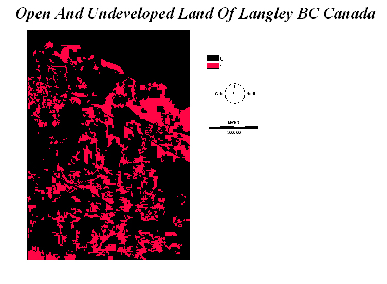
Open and Undeveloped Land Constraint:

           My second constraint was to build on open and undeveloped land within Langley, BC Canada. And so I reclassed the landuse map and selected 4 since it was open and undeveloped land according to the legend for the land-use.

Reclassed land-use for only open and undeveloped areas in Langley, BC Canada

1. Residential Land-Use:

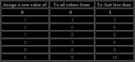
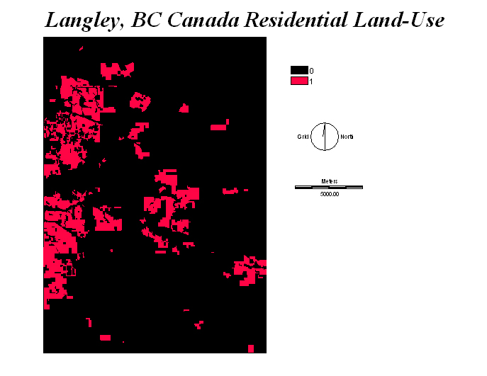
          One of my factors was distance from residential areas. And so I reclassed residential - single, residential - rural and residential - townhouses and low-rise apartments with a value of 1 and everything else a value of 0. Since Langley has a problem with youths riding pocket bikes in residential areas, I thought this would be a very significant factor as I would want my facility to be within close proximity to these youths and very accessible for everyone else around the GVRD.

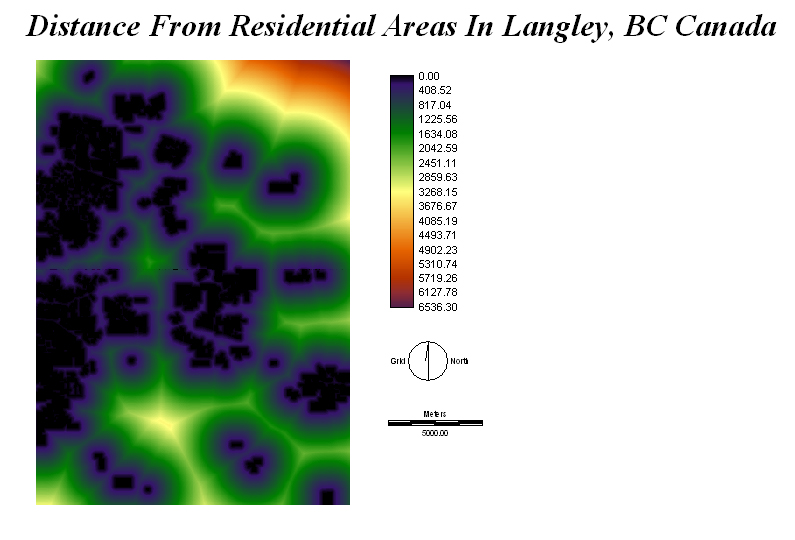
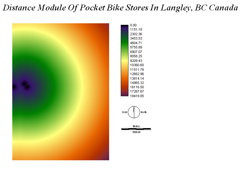
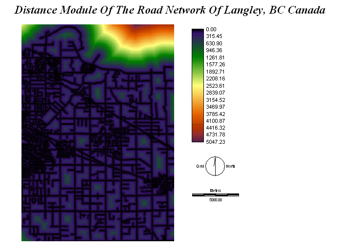
Reclassed land-use for all residential zones in Langley, BC Canada

           I then added a distance module to this new reclass of residential areas and labeled it "resdist." The distance module in IDRISI calculates the distance in meters from any locations selected in the reclass. The example would be these residential areas reclassed previously with a value of 1. The distance module will calculate the distance away from the residential areas and will display it in meters using a color range.

Distance module for residential zones

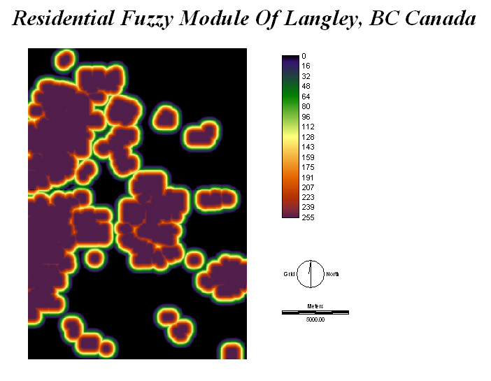
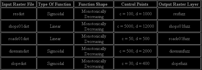
           After that, a fuzzy module was added next to the "resdist" file. I used a Monotonically Decreasing Sigmoidal function with control points a,b,c as 100 and control point d as 1000 to represent that areas within 100 meters is most suitable and will gradually become less suitable all the way up to 1000 meters. The fuzzy module is an operation that reclassifies a layer into 255 classes and it can be displayed in a color range. This module contains 4 control points labeled as A, B, C, D which will determine the type of graph when you add values to each of these control points.

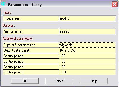
Using fuzzy module to create the residential fuzz

2. Pocket Bike Stores:

           One thing that I noticed when I imported the "stores" raster file is that the points don't show because they are so small.

Imported ASCII file of pocket bike stores into IDRISI

          Once I reclassed the stores and gave it a value of 1 for stores and 0 for the rest, I added a distance module which then showed the distance from these 3 points.

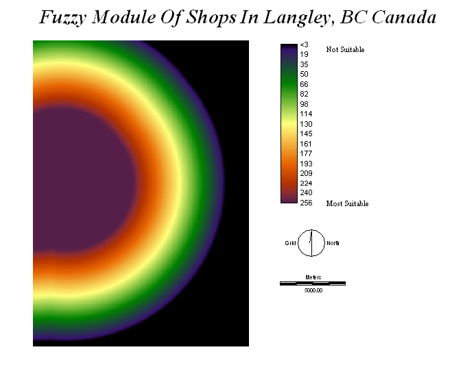
Using distance module on store locations in Langley, BC Canada

          A fuzzy module was then added in which I selected a Monotonically Decreasing Linear as the type of function to use with control points a,b,c as 5000 and control point d as 12000 in order to indicate that distances 5000 meters away from the store were the most suitable and as the distance increases all the way up to 12000 it was not suitable.

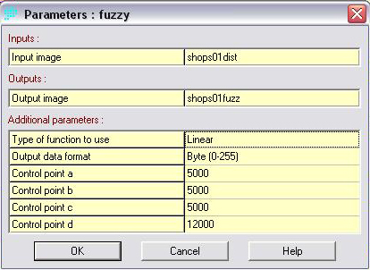
Using fuzzy module in order to create shop fuzz

3. Road Network:

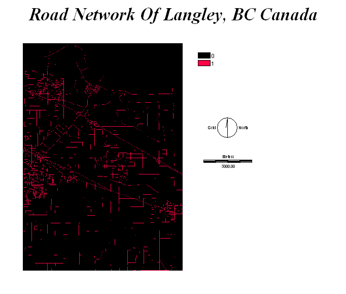
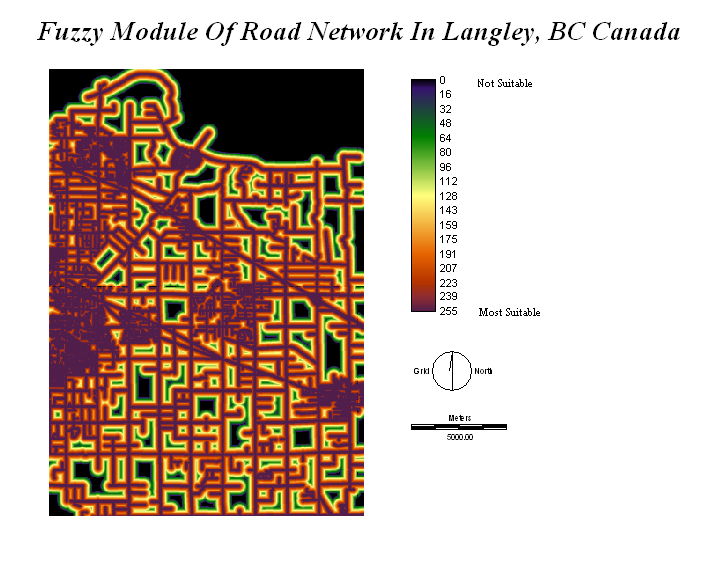
           The road network had to be reclassed with a value of 1 to represent all the road networks within Langley and a value of 0 for everything else that wasn't a road.

Reclass file for road networks

          Then a distance module was added and then a fuzzy module was added. I used a Monotonically Decreasing Linear type of function to use with control points a,b,c as 50 and control point d as 500. This indicated that the distances within 50 meters was suitable and extended all the way up to 500 meters which then was not suitable.

Using the distance module and then the fuzzy module to create road fuzz

4. Disenumeration Areas:

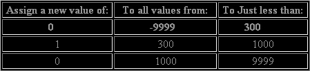
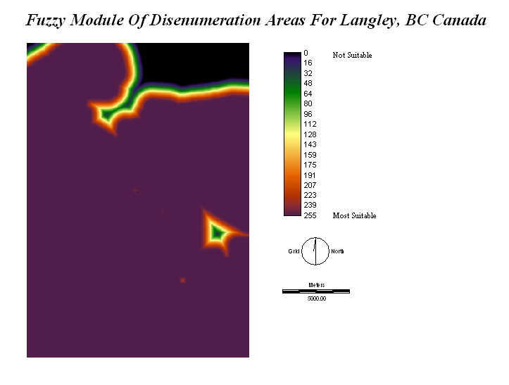
           I reclassed disenumeration areas from a population of 300 to 1000 because I wanted to select the average total population of Langley.

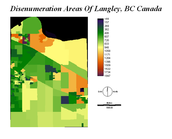
Disenumeration areas in Langley, BC Canada

          I also noticed that the areas that contained the highest population areas were on agricultural land which possibily could indicate that each farmer has several helpers to work on their farm land. I also wanted to locate my facility in an area that isn't highly dense because people from the rest of the GVRD will probably come to this facility and I don't require the need to have the highest total population to be surrounding my facility.

          After the distance module was applied, I put in the fuzzy module in which I selected the Monotonically Decreasing Sigmoidal type of function to use with the control points a,b,c as 500 and the control point d as 2000.

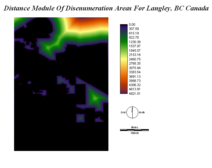
Using distance module and then the fuzzy module to create disenumeration fuzz

5. DEM - Slope:

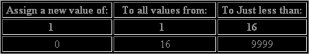
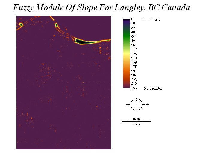
           The Surface Module was used for the DEM of Langley with a slope percentage of 15% because I wanted my facility to be built on any slope less than 15% so that it will be cheap and fairly flat to construct on. I then reclassed it for slope that is 15% and lower.

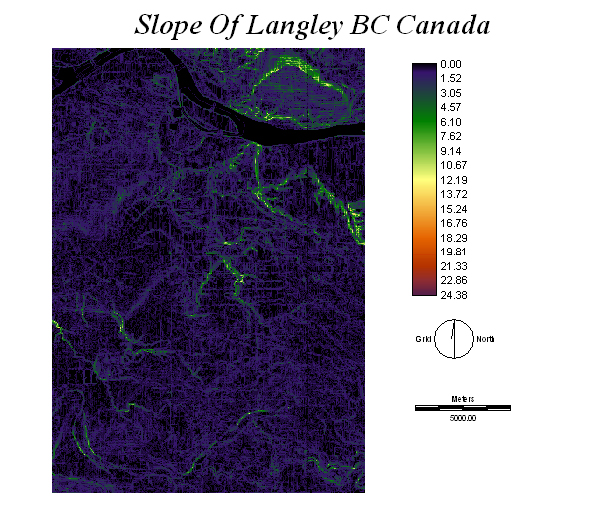
DEM using surface module showing slope 15% or less and reclassed into a value of 1

          After that a distance module was used and then a fuzzy module was added in which I used the Monotonically Decreasing Sigmoidal Type of function to use with control points a,b,c as 30 and control point d as 400 to indicate the areas within 30 metres of a 15% slope would be most suitable to build on and anything 400 meters away from a 15% slope would be not suitable.

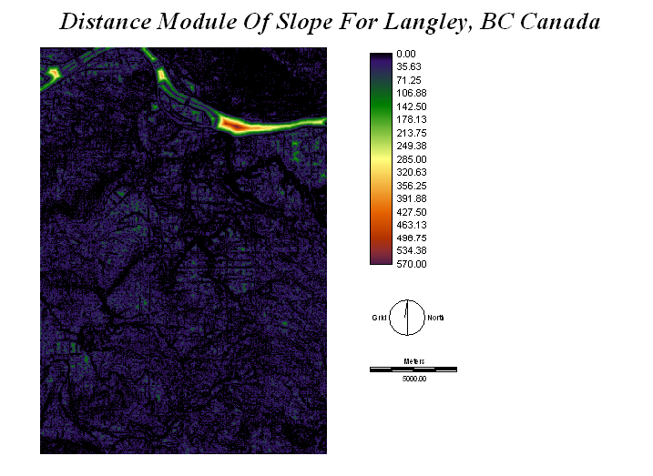
Using distance module and then the fuzzy module in order to create slope fuzz

 

Fuzzy Module Table:

          The program IDRISI contains only up to 255 classes for the RGB color spectrum. Therefore the fuzzy module operation is limited to this range from 0 to 255 classes when reclassing a layer such as the "distance" layer. And so, with the fuzzy module, there are 4 main control points which are classified as "a, b, c, d." There are different types of functions which produce different types of graphs which depend on the values that you enter for each control point. The types of functions include "Sigmoidal", "J-Shaped", "Linear" and "User-Defined". The simplist type would be the "Linear" function in which it represents an equal range when inputing the values of the control points. In my model, I assigned the "Linear" function to the road network and shops. The reason for this is that I wanted my facility to be at least 50 meters away from a road network but anything past 500 meters wouldn't be suitable. I know that people around the GVRD would probably drive to my facility so as long as the facility was 50 meters close to a road network it was fine and the range could range equally out to 500 meters. As for the shops, I wanted the facility to be as close as possible to the retail stores so I gave a big range of 5000 meters as the most suitable and the range could equally increase all the way out to 12000 meters where I thought would be too far and anything past it would be not suitable. The "Sigmoidal" function depending on where you set the control points can give out a steep slope. I decided to use tis function for slope, residential and disenumeration areas because I wanted to set a strict limit to each of these input files with the last control point D as the monotonically decreasing function shape which would be the limit where the area beyond this point would not be considered suitable. Therefore, I used monotonically decreasing function shapes for all my input files because I wanted my facility to be within all these parameters but with different ranges of distance for each of the input files. An example of this would be for the shops, the "shopdistance" has the function type linear with the shape monotonically decreasing. The control points were a = 5000, b = 5000, c = 5000, d = 12000 to represent that the facility would be most suitable within 5000 meters away from a retail shop. And anywhere past 5000 meters ranging all the way to 12000 meters would still be suitable as well but the distance to travel would be much greater. But once the distance reaches 12000 meters, anything beyond this distance would not be suitable. For the 255 colors in the fuzzy module, at point 255, it would represent the reclass distance of 5000 meters and then the range of the color spectrum would decrease to 0 where it would represent the reclass distance of 12000 meters which means that at 0, anything beyond this point would not be suitable.