Chapter Contents
Previous
Next
|
Chapter Contents |
Previous |
Next |
| Nonlinear Optimization Examples |

The following code calls the NLPTR subroutine to solve the optimization problem:
   proc iml;
      title 'Test of NLPTR subroutine: Gradient Specified';
      start F_ROSEN(x);
         y1 = 10. * (x[2] - x[1] * x[1]);
         y2 = 1. - x[1];
         f  = .5 * (y1 * y1 + y2 * y2);
         return(f);
      finish F_ROSEN;

      start G_ROSEN(x);
         g = j(1,2,0.);
         g[1] = -200.*x[1]*(x[2]-x[1]*x[1]) - (1.-x[1]);
         g[2] =  100.*(x[2]-x[1]*x[1]);
         return(g);
      finish G_ROSEN;

      x = {-1.2 1.};
      optn = {0 2};
      call nlptr(rc,xres,"F_ROSEN",x,optn) grd="G_ROSEN";
      quit;
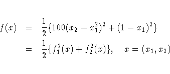
The NLPTR is a trust-region optimization method. The F_ROSEN module represents the Rosenbrock function, and the G_ROSEN module represents its gradient. Specifying the gradient can reduce the number of function calls by the optimization subroutine. The optimization begins at the initial point x=(-1.2 , 1). For more information on the NLPTR subroutine and its arguments, see the section "NLPTR Call". For details on the options vector, which is given by the OPTN vector in the preceding code, see the section "Options Vector".
A portion of the output produced by the NLPTR subroutine is shown in Figure 11.1.
Since f(x) = (1/2) {f12(x) + f22(x)}, you can also use least-squares techniques in this situation. The following code calls the NLPLM subroutine to solve the problem. The output is shown in Figure 17.5.
   proc iml;
      title 'Test of NLPLM subroutine: No Derivatives';
      start F_ROSEN(x);
        y = j(1,2,0.);
        y[1] = 10. * (x[2] - x[1] * x[1]);
        y[2] = 1. - x[1];
       return(y);
      finish F_ROSEN;

      x = {-1.2 1.};
      optn = {2 2};
      call nlplm(rc,xres,"F_ROSEN",x,optn);
      quit;
The Levenberg-Marquardt least-squares method, which is the method used by the NLPLM subroutine, is a modification of the trust-region method for nonlinear least-squares problems. The F_ROSEN module represents the Rosenbrock function. Note that for least-squares problems, the m functions f1(x), ... , fm(x) are specified as elements of a vector; this is different from the manner in which f(x) is specified for the other optimization techniques. No derivatives are specified in the preceding code, so the NLPLM subroutine computes finite difference approximations. For more information on the NLPLM subroutine, see the section "NLPLM Call".


The following code calls the NLPCG subroutine to solve the optimization problem. The infeasible initial point x0 = (-1,-1) is specified, and a portion of the output is shown in Figure 11.2.
   proc iml;
      title 'Test of NLPCG subroutine: No Derivatives';
      start F_BETTS(x);
         f = .01 * x[1] * x[1] + x[2] * x[2] - 100.;
         return(f);
      finish F_BETTS;

      con = {  2. -50.  .   .,
              50.  50.  .   .,
              10.  -1. 1. 10.};
      x = {-1. -1.};
      optn = {0 2};
      call nlpcg(rc,xres,"F_BETTS",x,optn,con);
      quit;
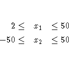
The NLPCG subroutine performs conjugate gradient optimization. It requires only function and gradient calls. The F_BETTS module represents the Betts function, and since no module is defined to specify the gradient, first-order derivatives are computed by finite difference approximations. For more information on the NLPCG subroutine, see the section "NLPCG Call". For details on the constraint matrix, which is represented by the CON matrix in the preceding code, see the section "Parameter Constraints".
| |||||||||||||||||||||||||||||||||||||||||||||||||||||||||||||||||||||||||||
| ||||||||||||||||||||||||||||||||||||||||||||||||||||||||||||||||||||||||||||||||||||||||||||||||||||||||||||||||||||||||||||||||||
Since the initial point (-1,-1) is infeasible, the subroutine first computes a feasible starting point. Convergence is achieved after three iterations, and the optimal point is given to be x* = (2,0) with an optimal function value of f* = f(x*) = -99.96. For more information on the printed output, see the section "Printing the Optimization History".


   proc iml;
      start F_HS43(x);
         f = x*x` + x[3]*x[3] - 5*(x[1] + x[2]) - 21*x[3] + 7*x[4];
         return(f);
      finish F_HS43;
      start C_HS43(x);
         c = j(3,1,0.);
         c[1] = 8 - x*x` - x[1] + x[2] - x[3] + x[4];
         c[2] = 10 - x*x` - x[2]*x[2] - x[4]*x[4] + x[1] + x[4];
         c[3] = 5 - 2.*x[1]*x[1] - x[2]*x[2] - x[3]*x[3]
                  - 2.*x[1] + x[2] + x[4];
         return(c);
      finish C_HS43;
      x = j(1,4,1);
      optn= j(1,11,.); optn[2]= 3; optn[10]= 3; optn[11]=0;
      call nlpqn(rc,xres,"F_HS43",x,optn) nlc="C_HS43";
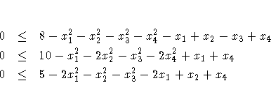
The F_HS43 module specifies the objective function, and the C_HS43 module specifies the nonlinear constraints. The OPTN vector is passed to the subroutine as the opt input argument. See the section "Options Vector" for more information. The value of OPTN[10] represents the total number of nonlinear constraints, and the value of OPTN[11] represents the number of equality constraints. In the preceding code, OPTN[10]=3 and OPTN[11]=0, which indicate that there are three constraints, all of which are inequality constraints. In the subroutine calls, instead of separating missing input arguments with commas, you can specify optional arguments with keywords, as in the CALL NLPQN statement in the preceding code. For details on the CALL NLPQN statement, see the section "NLPQN Call".
The initial point for the optimization procedure is x=(1,1,1,1), and the optimal point is x*=(0,1,2,-1), with an optimal function value of f(x*) = -44. Part of the output produced is shown in Figure 11.3.
| ||||||||||||||||||||||||||||||||||||||||||||||||||||||||||||||||||||||||||||||||||||||||||||||
| ||||||||||||||||||||||||||||||||||||||||||||||||||||||||||||||||||
In addition to the standard iteration history, the NLPQN subroutine includes the following information for problems with nonlinear constraints:
|
Chapter Contents |
Previous |
Next |
Top |
Copyright © 1999 by SAS Institute Inc., Cary, NC, USA. All rights reserved.